Screen reader users, click here to load entire articleThis
page uses JavaScript to progressively load the article content as a
user scrolls. Screen reader users, click the load entire article button
to bypass dynamically loaded article content.
Department of Physics, Hiroshima University, 1-3-1 Kagami-yama, Higashi-Hiroshima 739-8526, Japan
Received 13 June 2013
Revised 11 September 2013
Available online 9 October 2013
Highlights
•
Relativistic power-law densities admit a stable and extensive entropy functional.
•
Positive heat capacities and compressibility ensure their thermodynamic stability.
•
Quantization of nonthermal relativistic power-law ensembles in Fermi statistics.
•
Spectral fitting of nonthermal plasmas with ultra-relativistic power-law densities.
•
Entropy, temperature and chemical potential of the cosmic-ray electron/positron flux.
Abstract
Thermodynamically
stable ultra-relativistic power-law distributions are employed to model
the recently measured cosmic-ray electron flux and the positron
fraction. The probability density of power-law ensembles in phase space
is derived, as well as an extensive entropy functional. The phase–space
measure is transformed into a spectral number density, parameterized
with the Lorentz factor of the charges and quantized in Fermi
statistics. Relativistic power-law ensembles admit positive heat
capacities and compressibilities ensuring mechanical stability as well
as positive root mean squares quantifying thermodynamic fluctuations.
The wideband spectral fitting of dilute nonthermal electron–positron
plasmas with ultra-relativistic power-law densities is explained.
Keywords
Nonthermal power-law distributions;
Stability and extensivity of entropy;
Quantization of stationary non-equilibrium ensembles;
Hybrid quantum ensembles;
Ultra-relativistic electron–positron plasma;
Spectral fitting of a two-component plasma with power-law densities;
Cosmic-ray electron/positron flux
1. Introduction
We study nonthermal power-law ensembles capable of reproducing the flux of ultra-relativistic particles [1], [2], [3], [4] and [5]
such as cosmic-ray electrons and positrons. In particular, we derive
power-law distributions from empirical spectral fits which are
thermodynamically and mechanically stable, admitting positive heat
capacities and compressibilities. The entropy of power-law ensembles is
shown to be an extensive variable, and the positivity of the root mean
squares of thermodynamic variables is explicitly demonstrated, ensuring a
negative second entropy differential d2S≤0 subject to the extremal condition dS=0.
The
spectral number density of ultra-relativistic power-law ensembles
admits a convenient parameterization by the Lorentz factor of the
particles. We derive the classical number density from the phase–space
probability measure, which is taken as the starting point for the
quantization of classical power-law ensembles in Fermi statistics. We
also briefly outline the bosonic quantization of power-law densities as
well as the fermionic counterpart to electromagnetic gray-body
radiation, with Lorentz factors defined by group velocity in a
dispersive spacetime. Hybrid quantum distributions interpolating between
Fermi and Bose statistics are derived.
In Section 2,
we give an overview of the power-law densities studied, including their
partition function, the basic thermodynamic variables, their variances,
the equations of state, and show thermodynamic stability. In
Section 3,
we study classical power-law densities in phase space, their
probability density and entropy functional, fluctuations of internal
energy, particle number and entropy, as well as the quantization of
nonthermal power-law ensembles.
In Section 4,
we discuss wideband spectral fitting with ultra-relativistic power-law
densities. The power-law densities studied here are aimed at this
purpose, being thermodynamically stable empirical distributions
sufficiently general to reproduce the multiple spectral peaks of
broadband spectra. We show how to extract temperature, fugacity and
chemical potential, as well as the power-law amplitudes and exponents
from the measured particle flux. We also discuss energy scales and
conditions for the applicability of the classical limit of the
distributions.
In Section 5,
we perform a spectral fit to the cosmic-ray electron flux, employing an
ultra-relativistic classical power-law density. We use GeV data sets
collected with the PAMELA and Fermi satellites [6], [7] and [8], extended into the low TeV region by an atmospheric Cherenkov array [9], [10] and [11].
Based on the electronic number density (obtained from the spectral fit)
and the recently measured positron fraction, we calculate the spectral
number density of the cosmic-ray positron flux in the
1 GeV–3 TeV interval. Finally we estimate the specific energy
and number densities, as well as temperature and entropy production of
ultra-relativistic cosmic-ray electrons/positrons, which constitute a
nonthermal two-component plasma, dilute and at high temperature. In
Section 6, we present our conclusions.
2. Fermionic power-law distributions
2.1. General outline: spectral number density, partition function, entropy
Fermionic power-law ensembles are defined by the distributions (number densities)
parameterized by the Lorentz factor γ. The positive spectral function G(γ) in the denominator is normalized as G(1)=1 and is to be determined from a spectral fit. The mass parameter m is a shortcut for the rest energy mc2, so that E=mγ is the particle energy, and s is the spin multiplicity. The dimensionless temperature parameter is β=m/(kBT), with Boltzmann constant kB. The dimensionless real fugacity parameter α is related to the chemical potential μ by α=−βμ/m, and z=e−α is the fugacity. We specify G(γ) as a power-law ratio,
where δ is a real power-law exponent. The amplitudes ai,bi defining g(γ) are positive, and so are the exponents, 0<σ1<⋯<σn and 0<ρ1<⋯<ρk.
Empirical spectral functions of this type suitable to model multiple
spectral peaks in wideband spectra have been suggested in Refs. [1], [2] and [3], a specific choice of the ratio g(γ) is worked out in Sections 4 and 5. Fermionic power-law ensembles with g(γ)=1 have been studied in Refs. [12], [13], [14], [15] and [16], and thermodynamic stability of the ratios (2.2) is demonstrated in Section 2.2.
referring to particles with energies exceeding Ecut=mγcut, where γcut≥1 is the cutoff Lorentz factor. The partition function ZF is stated in (2.6). The ultra-relativistic limit of dρF(γ) is obtained by replacing in (2.1), which applies if γcut≫1. The thermal Fermi–Dirac distribution is recovered with δ=0,g(γ)=1 and γcut=1 as the lower integration boundary of the partition function. Here, we study nonthermal averages with real power-law index δ and empirical spectral function g(γ) extracted from spectral fits of measured flux densities.
The spectral number density (2.1) is based on the dispersion relation . The integration in momentum space is parameterized as , so that the particle density (2.1) is compiled as
Remark.
We may consider a more general dispersion relation, , with energy-dependent dimensionless permeabilities and resulting in a dispersive power-law density, a massive counterpart to photonic gray-body radiation. The integration in (2.3) is then over intervals in which the radicand of p(γ) is positive, and the normalization is done with the smallest possible Lorentz factor, instead of g(1). We still have γ=E/m, and the Lorentz factor γ can be parameterized by group velocity via m/υ=dp/dγ. Here, we use vacuum permeabilities, .
The internal energy (total energy of particles with Lorentz factor exceeding the lower threshold γcut) is
On introducing specific densities for the extensive variables, S/V,U/V and N/V, the volume factor drops out in (2.7), since logZF∝V, so that S is homogeneous. We can also replace the partition function in (2.7) by the pressure variable P,logZF=PVβ/m.
The classical limit of the partition function (2.6) is obtained by expanding the logarithm,
which is the classical limit of the spectral number density dρF in (2.1) and (2.2), apparently valid for . High- and low-temperature expansions of classical power-law ensembles based on dρB in (2.9) with g(γ)=1 and s=1 can be found in Ref. [12].
The spectral density of the non-relativistic Fermi gas,
is recovered by expanding the Lorentz factor in the power-law density (2.1) as γ=(1−υ2)−1/2≈1+υ2/2. The power-law factor G(γ) does not enter in leading order in the υ2 expansion, G(γ)∼1, and the rest mass can be absorbed in the fugacity, z0=e−α0,α0=α+β. The non-relativistic chemical potential μ0 is obtained by subtracting the rest mass from the relativistic potential, μ0=−α0m/β=μ−m. We find the particle count
The velocity parameter υ is dimensionless, measured in units of c. The classical Maxwell distribution is obtained by expanding the denominator of (2.10) and the logarithm in (2.12). The non-relativistic limit of the power-law densities (2.1) is always a thermal distribution, since G(γ)∼1 in leading order.
2.2. Thermodynamic stability: positivity of specific heat and compressibility
For the remainder of this section, we consider the classical limit based on the partition function (2.8) and density dρB in (2.9). In this limit, we can identify N=logZB, cf. (2.3), so that P=mN/(βV) is the thermal equation of state, cf. after (2.7). We may then explicitly solve (2.8) for α(β,N/V) and substitute this into the classical limit of the internal energy (2.5) and entropy (2.7) to obtain the U(β,N,V) and S(β,N,V) representations thereof:
As U∝N,
we find equipartition of energy even at stationary non-equilibrium. In
the low-temperature regime, the kinetic particle energy of an ideal gas
is recovered as leading order in a 1/β expansion, U/N−m∼(3/2)m/β.
The entropy (2.7) reads in the S(β,N,V) representation
with integral K(β) in (2.14). The free energy F(β,N,V) is found via (2.16) and (2.17), F=U−mS/(kBβ). The isothermal compressibility follows from the thermal equation of state,
and the adiabatic compressibility is calculated via the heat capacities, κS=κTCV/CP. Thus, if 0≤CV≤CP is satisfied, this also implies mechanical stability 0≤κS≤κT. The isochoric heat capacity is
Thus the stability criteria to guarantee d2S≤0 are satisfied, since (logK),β,β≥0 holds according to the Schwarz inequality (K,β)2≤KK,β,β.
Stability
implies well-defined positive standard deviations of the thermodynamic
variables. Temperature fluctuations are determined by the isochoric
specific heat,
where we can use the thermal equation of state to obtain the (β,N,V) representation thereof. Relative fluctuations such as scale with N−1/2. The variance of the chemical potential can be assembled as
with α in (2.13), U in (2.16) and CV in (2.19)
substituted. The variances of the extensive variables (internal energy,
particle count and entropy) will be derived in phase space, cf.
Section 3.2.
3. Power-law ensembles in phase space
3.1. Classical probability density
We give a probabilistic interpretation of the classical spectral number density dρB(γ) in (2.9). To this end, we consider the phase space of n particles with measure
where the d3qi integration is over a volume V, and the dγi integrations range in the interval γcut≤γi≤∞, cf. after (2.3). The angular integration over the solid angle dΩ has been carried out and gives the factor 4π. The scale factor (2πħ)3n renders the measure dimensionless. The probability density on the n-particle states factorizes as
The factor 1/n! accounts for indistinguishability and the positive integer s for spin multiplicity. The normalization factor ξ included in the weight bn(p,q) is found by summation over the n-particle subspaces,
We use the shortcut ξ=logZB and the general identity ZB,β,α/ZB=ξ,β,α+ξ,βξ,α as well as the special properties ξ,α=−ξ and N=ξ(β,α,V). Thus, 〈n〉=N and 〈n2〉=N(N+1), keeping the volume V constant in contrast to the fluctuating particle number N.
so that 〈un〉=(1+N)U. The standard deviations are readily assembled with the expectation values , and (3.8). Defining Δn=n−〈n〉, etc., we find the covariance matrix elements as
where ξ=logZB is the classical partition function (2.8). This is identical to the entropy S(β,α,V) stated in (2.7), according to the averages (3.5) and and the normalization (3.3). We regard (3.13) as the expectation value of , and use the correlations (3.9) to assemble 〈s2〉 and the entropy variance
Here, we can substitute α(β,N/V) in (2.13), U(β,N) in (2.16) and CV(β,N) in (2.19) to obtain the (T,N,V)
representation of the fluctuations. Alternatively, we may obtain the
entropy fluctuations by making use of error propagation. To this end, we
employ the S(U,N,V) representation, obtained by substituting α=α(U,N,V),β=β(U,N,V) (implicitly defined by (2.3) and (2.5)) into (2.7). The entropy variance (3.14) is recovered via
A basis |n〉 for the occupation number representation of the fermionic creation and annihilation operators (labeled by the wave vector of the modes) can be found in Ref. [17]. The particle number operator is , where . The energy operator is , where . The power-law weight factor hn(p,q) of the classical probability density in (3.2) is quantized as , , where . The energy operator is dimensionless, rescaled with the particle mass. is the Lorentz factor parameterized with the wave vector, and m stands for mc2. In the occupation number representation, the Hermitian number operators are diagonal, , and the fermionic occupation number attached to a wave vector can only take the values zero and one. (In the bosonic case sketched below, ranges between zero and infinity.) We also note the dispersion relation , relating electron energy and wave number . Finally, is the wave number of the lower energy threshold ħωcut=mγcut. Integration over wave vectors is defined by d3k=d3p/ħ3, with the momentum-space measure d3p parameterized by the Lorentz factor as in (3.1).
We employ box quantization, discretizing the wave vector as , so that summations are taken over integer lattice points in R3, corresponding to periodic boundary conditions on a box of size V=L3. By making use of , we can write trace (3.16) over the basis |n〉 as
The continuum limit L→∞ amounts to replacing the summation over the lattice wave vectors by the integration , where the factor s accounts for spin degeneracy,
Introducing the Lorentz factor γ as integration variable, , we arrive at the partition function logZF stated in (2.6).
We outline quantization of relativistic power-law ensembles in Bose–Einstein statistics [17], [18] and [19]. In this case, the summation over the occupation numbers in (3.17) extends to infinity,
which differs from the fermionic density dρF(γ) in (2.1) only by the minus sign in the denominator. s is a multiplicity index, and G(γ) is the spectral function (2.2). In the bosonic case, the reciprocal spectral function G−1(γ) must be bounded, its maximum being attained at γc. (γc can be infinite.) The fugacity z=e−α is restricted by z≤zc=G(γc), so that the denominator in (3.24) is positive. The classical regime is , whereas quantum condensation effects arise in the opposite limit, .
3.4. Hybrid quantum statistics
We briefly discuss hybrid distributions, in which the fermionic exclusion principle is softened to allow Nid identical particles labeled by the same wave vector . The partition function interpolating between Fermi and Bose statistics is found by extending the summation in (3.17),
where the allowed multiplicity of particles in identical states is an arbitrary positive integer Nid. Summation of the finite geometric series in (3.25) gives
The Fermi–Dirac and Bose–Einstein partitions logZF in (2.6) and logZE in (3.22) are recovered for Nid=1 and Nid=∞, respectively. The spectral density dρH(Nid)(γ) of a hybrid quantum ensemble of fixed multiplicity Nid can be identified as in and via the particle count,
The limit Nid→∞ can be carried out in this representation of dρH(Nid)(γ), provided that βγ+α+logG(γ)>0, cf. after (3.24). Even if this constraint is not met, the positivity of density (3.29) is obvious in the equivalent representation
irrespective of the (finite) multiplicity Nid and the sign of exponent βγ+α+logG(γ), and dρH(Nid)(γ) stays finite when this exponent approaches zero. Alternatively, we may write the hybrid density (3.30) as
so that 0<dρH(Nid)(γ)<dρH(Nid+1)(γ) is evident, cf. after (3.26), which holds for arbitrary real exponents βγ+α+logG(γ). In contrast to the Bose–Einstein limit Nid=∞, there is no constraint on the fugacity parameter α resulting in a condensed phase, so that the reciprocal spectral function 1/G(γ) need not be bounded in hybrid statistics, even for high multiplicity, so long as Nid is finite.
Remarks.
To check the stability of the above quantum
densities, one starts with the high- and low-temperature asymptotics of
the thermodynamic variables, which can be done analytically in leading
order [13] and [14].
To check positivity of the specific heat and compressibility in the
intermediate temperature regime, one has to specify the input parameters
and study the cross-over numerically, in contrast to the classical
variables discussed in Section 2.2.
If positivity turns out to be violated for certain parameter ranges,
the respective intervals have to be excluded. I also note that the
power-law factor G(γ)
drops out in the non-relativistic limit also in the quantum
distributions, and has a pronounced effect only for large Lorentz
factors, so that their applicability is currently limited to
astrophysical plasmas. Whether the hybrid densities (3.29) can be related to real systems remains to be seen. The spectral fits in Section 5 are performed with the classical density (2.9).
4. Nonthermal spectral fitting in the ultra-relativistic regime: How to set it up in practice
with γ=E/m, where m stands for mc2, and use dimensionless quantities: E and m in units of , where the factor 103d (usually with integer d)
allows us to conveniently shift the energy scale. The units chosen for
length, time and temperature are meter, second and Kelvin, so that and . Finally, β=m/(kBT), with and . The contribution of the Coulomb interaction [20], [21] and [22] to the partition function is negligible in the case of a dilute ultra-relativistic plasma at high temperature, since e2/(4πrkBT)≪1, with interparticle distance r=(N/V)−1/3 and fine-structure constant e2/(4πħc)≈1/137 (Heaviside–Lorentz system), cf. Table 1.
Table 1.
Thermodynamic parameters of the ultra-relativistic electron/positron distributions dρB/dE in (5.3), extracted from the spectral fit of the electron flux Fe(E) in (5.4) and the positron flux Fp(E) in (5.7), cf. Fig. 1 and Fig. 2. N/V is the specific number density and U/V the specific energy density calculated via (4.12) with lower cutoff energy . Recorded are temperature T, fugacity z and chemical potential μ, cf. (4.11), as well as the specific entropy density S/V scaled with the Boltzmann constant, cf. (4.14). The entropy production is mainly due to the fugacity term in (4.14). For comparison, the specific entropy density of the cosmic microwave background is .
The first row of the table refers to cosmic-ray electrons with energies
above 1 GeV (lower energy threshold of the observed flux), the
second to positrons.
If we use constant or dispersive permeabilities differing from 1, cf. the Remark after (2.4), we define the scaling function as , where γmin is the smallest Lorentz factor admissible in the dispersion relation. The fermionic spectral number density (4.1) reads in dimensionless quantities
where dΩ is the solid angle increment and dρF/dE the particle density (4.4). Density F(E) is the spectral number flux; the spectral energy flux is obtained by rescaling F(E) with E. To avoid steep spectral slopes in log–log plots, which tend to conceal the fine-structure, it is convenient to rescale F(E) with a suitable power Ek, where k is usually integer. (We will use k=3 in Section 5.) In dimensionless quantities, cf. (4.4) and (4.6),
s is the spin multiplicity. The classical flux FB(E) (defined by the Boltzmann density dρB/dE substituted in (4.6)) is found by dropping the ξ0 term in the denominator of (4.7),
with positive amplitudes and real exponents ηi,κi
(determining location, height and the two power-law slopes of each
peak) to be extracted from the spectral fit. Once the exponents and
amplitudes on the right-hand side of (4.10) are known, the power-law ratio fB(E) in (4.3) is unambiguously defined. The amplitude and the exponent 2+k−δ can readily be identified as well, by considering the limit E→0 in (4.10).
Remark.
The individual spectral components of
nonthermal high-energy spectra are typically composed of a power-law
ascent, followed by a slightly curved descending power-law slope due to
an exponential cutoff [15] and [16]. Power-law slopes are linear in log−log
plots, clearly distinguishable from curved exponential cutoffs, and
wideband spectra can readily be assembled with them. The power-law
slopes are often blurred due to overlapping spectral peaks. The spectral
function (4.10)
models a sequence of such spectral peaks. Given that spectral fits are
usually performed in double logarithmic representation, power-law ratios
of type (2.2) and (4.3) seem to be sufficiently general, although more complicated spectral functions have been considered [2]. The spectral functions (2.2) are constant for small Lorentz factors, g(γ→1)∼1, and have a power-law shape in the opposite limit, g(γ→∞)∝γσn−ρk. A different cross-over (other than in (2.2)) does not affect the thermodynamic stability, cf. Section 2.2, but if one replaces, for instance, the denominators in (4.10) by , it would not be possible to fit the electron spectrum in Fig. 1.
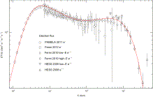
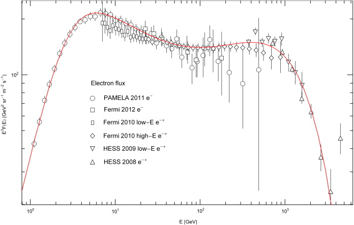
Fig. 1.
Cosmic-ray
electron flux. Data points from PAMELA 2011 (magnetic spectrometer
combined with calorimeter for bremsstrahlung showers, pure electron
flux) [6], Fermi LAT 2012 (Large Area pair-conversion γ-ray Telescope, pure electron flux) [7], Fermi LAT 2010 (combined electron–positron flux) [8],
HESS 2009 (High-Energy Stereoscopic System, an imaging atmospheric
Cherenkov telescope, low-energy component of combined electron–positron
flux) [10], and HESS 2008 (high-energy component of combined electron–positron flux) [11].
The low-energy Fermi LAT 2010 data are not included in the fit, as they
are not compatible with the overlapping PAMELA flux, which has smaller
error bars in this region. The fit does not discriminate between pure
electron and combined electron–positron data points. (The Fermi 2012
pure electron data are quite comparable to the Fermi 2010 combined
electron–positron data, in fact intersecting them. The Fermi 2010
low-energy flux is a combined electron–positron flux, whereas the
overlapping PAMELA flux has a noticeably higher intensity even though it
is a pure electron flux.) The solid curve is a plot of the
ultra-relativistic nonthermal electron flux Fe(E) (spectral number-flux density, scaled with E3 in the figure) stated in (5.4); the fitting parameters in (5.1) and (5.2) can be read off from the analytic representation of E3Fe(E) in (5.4). The thermodynamic parameters of the electronic power-law distribution (5.3) generating the depicted flux density are listed in Table 1.
Here, ξ0≈3.18×10⁻⁹(d+6)(2/s), which becomes moderate on the 10−9 eV scale (d=−6), cf. (4.8) and after (4.1), and m≈0.511×10⁻³(d+1) for an electron/positron gas. The specific particle density N/V in (2.3) reads in dimensionless quantities
where the lower cutoff energy is related to the Lorentz factor by Ecut=mγcut. The energy density , cf. (2.5), is obtained by adding a factor E to the integrand in (4.12). (These integrals are numerically very tame.) The specific densities N/V and U/V become independent of the particle rest mass m in the ultra-relativistic regime , since the roots in (4.12) and (4.13) can be dropped, so that the mass is completely absorbed in the fitting parameters. The classical limit of the particle density N/V is found by putting the term in the denominator of the integrand in (4.12) to zero. Since ξ0 is extremely small on the GeV scale and the amplitude (extracted from the spectral fit) turns out to be moderate, we can safely assume and use the classical limit. Expanding the logarithm in the partition function (4.13) in leading order in , we recover N=logZB, cf. before (2.13). The entropy density (2.7) can be assembled from the classical specific number and energy densities in (4.12),
where we have put α=−logz in (2.7). Fugacity and temperature are extracted from the fitting parameters by way of (4.11).
As mentioned, in the ultra-relativistic limit, we do not need to know
the mass of the particles to calculate the specific particle and energy
densities (4.12) from the spectral fit. However, the particle mass affects the entropy density via the fugacity, cf. (4.11),
as the entropy depends on the zero point of the chemical potential.
This zero point is determined by the normalization of the spectral
function G(γ) in (2.1) at γ=1. We have chosen G(1)=1, so that the chemical potential of the non-relativistic Fermi gas limit is recovered from the relativistic potential μ in (4.11) by subtraction of the rest mass, cf. after (2.10).
5. Spectral flux densities and thermodynamic parameters of cosmic-ray electrons/positrons
The spectral fits in Fig. 1 and Fig. 2 are performed with the classical ultra-relativistic flux density FB(E) in (4.9) and the spectral function fB(E) in (4.3). We employ a GeV energy scale (d=0, cf. after (4.1)), and scale the flux density with E3, cf. (4.9),
The fitting parameters in (5.1) are the power-law exponents δ,σ,ρ and amplitudes , as well as the exponent determining the cutoff. The ultra-relativistic limit applies, since the fit is done above a cutoff energy Ecut where m2/E2≪1. (We use Ecut≈1 on the GeV scale.) In this limit, the mass-square m2 is not a fitting parameter, as it is absorbed in the amplitudes . The classical spectral particle density reads, cf. (4.4) and (4.12),
The root can be dropped in the ultra-relativistic regime, and , cf. (4.2), (4.8) and (4.11). The spin multiplicity is s=2.
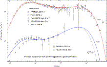
Fig. 2.
Cosmic-ray positron spectrum inferred from the measured electron flux and the positron fraction. The electron flux Fe(E) (upper solid curve, a plot of E3Fe(E) in (5.4)) is the same as in Fig. 1, on a compressed flux scale. The dotted curve labeled is the positron flux (5.6) assembled from the depicted fit Fe(E) of the electron flux and the analytic AMS fit of the positron fraction [23] stated in (5.5). The AMS positron fraction has been measured only up to 300 GeV, cf. Fig. 3, so that the dotted curve above this energy is an extrapolation based on the analytic ratio in (5.5). The solid curve Fp(E) is the predicted positron flux stated in (5.7), obtained by approximating below 300 GeV by a nonthermal power-law density analogous to the electronic flux density Fe(E). The positronic fitting parameters can be read off from E3Fp(E) in (5.7), and the thermodynamic parameters of the positron flux are recorded in Table 1. The depicted positron data from PAMELA 2013 [24]
and HEAT (High-Energy Antimatter Telescope, a balloon-born
superconducting magnet spectrometer with calorimeter and scintillation
counters attached) [29] have not been used in the derivation of the positronic flux density.
The parameters in (5.1) and (5.2) can be read off from this equation. The positron fraction Rp(E)=Fp/(Fe+Fp), where Fp(E) denotes the positronic flux density, was measured by the AMS Collaboration [23], cf. Fig. 3, without disentangling the electron and positron flux, and an analytic fit of the positron fraction was derived,
where E is in GeV units. Combining the electronic flux density (5.4) with the AMS ratio (5.5), we find an analytic representation of the positron flux,
This is a power-law fit to E3FAMSp(E) as defined by (5.6) with Fe(E)Fe(E) in (5.4) and RAMSp(E) in (5.5). In Fig. 3, we plot the positron fraction Rp(E)=Fp/(Fe+Fp)Rp(E)=Fp/(Fe+Fp), now directly calculated with the electronic/positronic power-law densities Fe(E)Fe(E) in (5.4) and Fp(E)Fp(E) in (5.7), and compare it to the analytic fit RAMSp(E) of the AMS data in (5.5). The thermodynamic parameters of the nonthermal electron–positron plasma are listed in Table 1, extracted from the flux densities Fe,p(E)Fe,p(E) in (5.4) and (5.7).
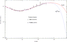
Fig. 3.
Positron fraction. Data points from AMS-02 2013 (Alpha Magnetic Spectrometer) [23] and PAMELA 2013 [24]. The dotted curve depicts the analytic fit RAMSp(E) obtained in Ref. [23], cf. (5.5). Above 300 GeV, RAMSp(E) is an analytic extrapolation, a plot of the AMS ratio (5.5). The solid curve Rp(E)Rp(E) is the positron fraction Fp/(Fe+Fp)Fp/(Fe+Fp) calculated from the electron flux Fe(E)Fe(E) in (5.4) (obtained from the fit in Fig. 1) and the positron flux Fp(E)Fp(E) in (5.7). The latter is found by approximating the AMS flux FAMSp(E) below 300 GeV by a nonthermal classical power-law density, cf. Fig. 2. The depicted exponential decay of the analytic AMS fraction RAMSp(E) is intermediate, terminating at about 10 TeV (with subsequent power-law decay according to (5.5)), in contrast to the predicted positron fraction Rp(E)=Fp/(Fe+Fp)Rp(E)=Fp/(Fe+Fp), whose exponential decay is final, determined by the temperature of the electron/positron flux densities in (5.4) and (5.7).
The
goal is to find power-law densities suitable for ultra-relativistic
wideband fitting. A consistent thermodynamic formalism requires these
distributions to admit an extensive and stable entropy functional
resulting in thermodynamic variables with positive standard deviations
and relative fluctuations vanishing in the thermodynamic limit. Here, we
have discussed a class of stable power-law densities, stationary
non-equilibrium distributions defined by an empirical spectral function,
a power-law ratio to be inferred from measured flux densities, cf.
Sections 2 and 3.
We explained the spectral fitting with ultra-relativistic power-law densities, cf. Section 4, and applied it to cosmic-ray electrons treated as dilute nonthermal plasma, cf. Section 5. The cosmic-ray electron flux as well as the AMS and PAMELA positron fraction [23] and [24]
are highly isotropic. The statistical description given here does not
involve any hypothetical assumptions on isotropically distributed
electron/positron sources and production mechanisms. The power-law
densities are empirically determined from spectral fits [25], [26], [27] and [28].
Cosmic-ray
electrons/positrons constitute a dilute nonthermal two-component
plasma, whose components can efficiently be modeled as classical
ultra-relativistic power-law ensembles. The classical limit allows
fairly explicit evaluation of the thermodynamic functions in (T,N,V)
representation. High-temperature expansions are not efficient though,
as they cannot adequately describe peak-to-peak cross-overs in wideband
spectra. The electron and positron spectra in Fig. 1 and Fig. 2
are not wideband, extending from the low GeV to the low TeV region, but
there are still two spectral peaks discernible, and the cross-over is
beyond asymptotic expansions.
The
cosmic-ray electron spectrum is well covered by several measurements in
the GeV and low TeV range. Once the power-law fit of the spectral
electron density is performed, cf. Fig. 1, it can be combined with the measured positron fraction, cf. Fig. 3, to obtain an estimate of the positronic flux density [24] and [29].
The positron flux is modeled by a nonthermal power-law density composed
of two spectral peaks like the electronic counterpart, cf. Fig. 2.
The thermodynamic parameters of the electron/positron gas can be read
off from the spectral fits. The temperature of the two non-equilibrated
components is comparable but decidedly different, and their specific
energy, entropy and number densities differ by roughly one order,
cf. Table 1.


 . Recorded are temperature T, fugacity z and chemical potential μ, cf. (4.11), as well as the specific entropy density S/V scaled with the Boltzmann constant, cf. (4.14). The entropy production is mainly due to the fugacity term in (4.14). For comparison, the specific entropy density of the cosmic microwave background is
  .
The first row of the table refers to cosmic-ray electrons with energies
above 1 GeV (lower energy threshold of the observed flux), the
second to positrons.
.
The first row of the table refers to cosmic-ray electrons with energies
above 1 GeV (lower energy threshold of the observed flux), the
second to positrons.


 is the positron flux (5.6) assembled from the depicted fit Fe(E) of the electron flux and the analytic AMS fit
  of the positron fraction [23] stated in (5.5). The AMS positron fraction
  has been measured only up to 300 GeV, cf. Fig. 3, so that the dotted curve
  above this energy is an extrapolation based on the analytic ratio
  in (5.5). The solid curve Fp(E) is the predicted positron flux stated in (5.7), obtained by approximating
  below 300 GeV by a nonthermal power-law density analogous to the electronic flux density Fe(E). The positronic fitting parameters can be read off from E3Fp(E) in (5.7), and the thermodynamic parameters of the positron flux are recorded in Table 1. The depicted positron data from PAMELA 2013 [24]
and HEAT (High-Energy Antimatter Telescope, a balloon-born
superconducting magnet spectrometer with calorimeter and scintillation
counters attached) [29] have not been used in the derivation of the positronic flux density.
below 300 GeV by a nonthermal power-law density analogous to the electronic flux density Fe(E). The positronic fitting parameters can be read off from E3Fp(E) in (5.7), and the thermodynamic parameters of the positron flux are recorded in Table 1. The depicted positron data from PAMELA 2013 [24]
and HEAT (High-Energy Antimatter Telescope, a balloon-born
superconducting magnet spectrometer with calorimeter and scintillation
counters attached) [29] have not been used in the derivation of the positronic flux density.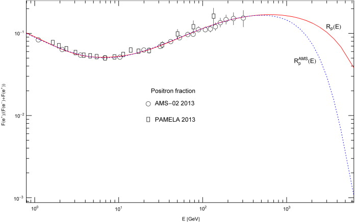

")

