
Tachyonic quantum densities of relativistic electron plasmas: Cherenkov spectra of γ-ray pulsars


- DOI: 10.1016/j.physleta.2014.06.005
- Get rights and content
Highlights
- •
-
Quantized tachyonic Cherenkov densities lead to subexponential spectral decay.
- •
-
γ -Ray spectral fits to Crab pulsar, PSR J1836+5925, PSR J0007+7303, PSR J2021+4026.
- •
-
The polarization of γ-rays is analyzed in the quasiclassical regime and quantum limit.
- •
-
Three degrees of polarization due to the negative mass-square of the Maxwell–Proca field.
- •
-
Weibull decay of spectral tails caused by frequency scaling of the tachyon mass.
Abstract
Tachyonic Cherenkov radiation in second quantization can explain the subexponential spectral tails of GeV
γ -ray
pulsars (Crab pulsar, PSR J1836+5925, PSR J0007+7303, PSR J2021+4026)
recently observed with the Fermi-LAT, VERITAS and MAGIC telescopes. The
radiation is emitted by a thermal ultra-relativistic electron plasma.
The Cherenkov effect is derived from a Maxwell–Proca field with negative
mass-square in a dispersive spacetime. The frequency variation of the
tachyon mass results in
![]() attenuation of the asymptotic Cherenkov energy flux, where
attenuation of the asymptotic Cherenkov energy flux, where
![]() is a decay constant related to the electron temperature and
ρ is the frequency scaling exponent of the tachyon mass. An exponent in the range
0<ρ<1 can reproduce the observed subexponential decay of the energy flux. For the Crab pulsar, we find
ρ=0.81±0.02,
inferred from the substantially weaker-than-exponential decay of its
spectral tail measured by MAGIC over an extended energy range. The
scaling exponent ρ determines whether the group velocity of the tachyonic
γ-rays is sub- or superluminal.
is a decay constant related to the electron temperature and
ρ is the frequency scaling exponent of the tachyon mass. An exponent in the range
0<ρ<1 can reproduce the observed subexponential decay of the energy flux. For the Crab pulsar, we find
ρ=0.81±0.02,
inferred from the substantially weaker-than-exponential decay of its
spectral tail measured by MAGIC over an extended energy range. The
scaling exponent ρ determines whether the group velocity of the tachyonic
γ-rays is sub- or superluminal.
Keywords
- Quantized tachyonic Cherenkov densities;
- Frequency-dependent tachyon mass;
- Superluminal radiation in a permeable spacetime;
- Transversal/longitudinal Cherenkov energy flux;
- Tachyonic spectral fits to γ-ray pulsars;
- Subexponential Weibull decay of spectral tails
1. Introduction
Stunning high-precision spectra of several γ-ray pulsars which defy traditional radiation models have recently been recorded by the Fermi satellite and the terrestrial γ-ray telescopes MAGIC and VERITAS. An account of these developments can be found in the review [1]. These spectra are difficult to explain, as the spectral tails decay more slowly than an exponential cutoff but faster than a power law, so that something in between these two extremes is needed.
Here, we will show that a Weibull [2] decay factor exp(−(E/E0)δ), 0<δ<1, in the asymptotic energy flux can reproduce the very accurately measured subexponential decay of the spectral tails. To this end, we will perform spectral fits to four Fermi-LAT pulsars (including the Crab pulsar), covering a representative range of shape parameters δ . First, however, we have to find a radiation model which produces an energy flux admitting asymptotic Weibull decay; this is the principal aim of this article. Time-honored electromagnetic radiation mechanisms such as inverse-Compton scattering or synchrotron and curvature radiation result in straight exponential cutoffs (δ=1) if the cross-section or radiation density is averaged over a relativistic equilibrated or non-thermal electronic source plasma.
We will invoke the tachyonic Cherenkov effect based on a Maxwell–Proca field theory with negative mass-square, and demonstrate that the Cherenkov flux density produced by an ultra-relativistic electron population decays subexponentially. This holds true in the quasiclassical regime as well as in the extreme quantum limit of the Cherenkov flux, with different shape parameters δ in the Weibull exponential. The spectral fits to the GeV pulsar spectra will be performed in the semiclassical regime, but the quantum limit is inescapable at sufficiently high frequency and can be manifested in TeV γ-rays.
Apart from subexponential Weibull decay, which is the main focus, there are also other features of tachyonic Cherenkov radiation quite different from electromagnetic radiation. For instance, three degrees of polarization, two transversal and one longitudinal due to the tachyonic mass-square of the radiation field. The Cherenkov emission angles differ for transversal and longitudinal γ-rays. Most importantly, the γ-rays can have a slightly superluminal group velocity depending on the Weibull shape parameter δ, and we will illustrate this with a pulsar spectrum.
In Section 2, we introduce the Lagrangian of the underlying field theory, a Proca field with negative mass-square, coupled to dispersive permeability tensors and an external spinor current. We discuss tachyonic radiation densities in second quantization, their polarization components and the effect of electron spin. We determine the frequency intervals in which Cherenkov radiation from an inertial Dirac electron current is possible, depending on the permeabilities in the Lagrangian and the electronic Lorentz factor, and derive the Cherenkov emission angles. The quantized electromagnetic Cherenkov densities [3], [4], [5], [6] and [7] are recovered in the limit of zero tachyon mass, and the classical tachyonic radiation densities [8] and [9] for small tachyon–electron mass ratio.
To relate the tachyonic Cherenkov densities to pulsar spectra, we have to average them over a relativistic electron plasma, cf. Section 3. We consider thermal equilibrium distributions as well as non-thermal power-law distributions for the radiating electron populations of the pulsars. The averaged differential flux densities are then fitted to the measured GeV pulsar spectra. There is a longitudinal radiation component, which is even more intense than the linearly polarized transversal radiation in the semiclassical regime. A second transversal degree of polarization emerges in the quantum regime, where the longitudinal energy flux weakens.
In Section 4, we study tachyonic flux densities in the quasiclassical regime. We explain the frequency variation of the tachyon mass and the tachyonic fine-structure constant, specializing to permeability tensors which give identical dispersion relations and group velocities for transversal and longitudinal quanta. Whether the group velocity is sub- or superluminal depends on the frequency variation of the tachyon mass, which is inferred from the decaying spectral tails of the pulsars.
In Section
5, we test the averaged tachyonic Cherenkov densities by performing spectral fits to the
γ -ray pulsars PSR
J1836+5925, PSR
J0007+7303, PSR
J2021+4026 and the Crab pulsar
[10] and [11]. In this way, the scaling exponent
ρ of the frequency-dependent tachyon mass
∝ωρ can be inferred. The decay of the spectral tails is weaker than exponential because of the Weibull decay factor
![]() ,
0<ρ<1, in the asymptotic flux density, the decay exponent
,
0<ρ<1, in the asymptotic flux density, the decay exponent
![]() being related to the temperature of the ultra-relativistic electron
plasma and the tachyonic mass amplitude. (The above mentioned Weibull
slope is thus
δ=1−ρ.) For
ρ<1/2, the radiation is superluminal
[12] and [13], as happens for pulsar PSR
J1836+5925. In the case of the Crab pulsar, the tachyon mass admits a scaling exponent
ρ
close to one, so that the Weibull exponential approximates power-law
decay of the spectral tail, and the radiation is slightly subluminal
despite of the tachyonic mass-square in the dispersion relations, cf.
Section 6.
Apart from the tachyonic Cherenkov effect discussed here, the
thermodynamics of superluminal signal transfer has been studied in Ref.
[14], electromagnetic radiation by acceleration of superluminal charges in Ref.
[15], and Cherenkov radiation from superluminally rotating light spots in Ref.
[16].
being related to the temperature of the ultra-relativistic electron
plasma and the tachyonic mass amplitude. (The above mentioned Weibull
slope is thus
δ=1−ρ.) For
ρ<1/2, the radiation is superluminal
[12] and [13], as happens for pulsar PSR
J1836+5925. In the case of the Crab pulsar, the tachyon mass admits a scaling exponent
ρ
close to one, so that the Weibull exponential approximates power-law
decay of the spectral tail, and the radiation is slightly subluminal
despite of the tachyonic mass-square in the dispersion relations, cf.
Section 6.
Apart from the tachyonic Cherenkov effect discussed here, the
thermodynamics of superluminal signal transfer has been studied in Ref.
[14], electromagnetic radiation by acceleration of superluminal charges in Ref.
[15], and Cherenkov radiation from superluminally rotating light spots in Ref.
[16].
2. Quantized tachyonic Cherenkov densities of relativistic electrons
The Cherenkov radiation densities stated below are derived from the Lagrangian [9]

The external current
![]() is generated by a uniformly moving subluminal charge
q with mass m and Lorentz factor
γ .
When quantizing, we use an inertial Dirac current. The Cherenkov
emission of the charge has two transversal and one longitudinal
polarization components. The spectral densities in second quantization
read, for the two linear transversal polarizations,
is generated by a uniformly moving subluminal charge
q with mass m and Lorentz factor
γ .
When quantizing, we use an inertial Dirac current. The Cherenkov
emission of the charge has two transversal and one longitudinal
polarization components. The spectral densities in second quantization
read, for the two linear transversal polarizations,


The zeros of the argument
![]() in the Heaviside function, cf.
(2.9), determine the frequency intervals (at fixed
γ ) in which
in the Heaviside function, cf.
(2.9), determine the frequency intervals (at fixed
γ ) in which
![]() , i.e. the transversal and longitudinal spectrum radiated by an inertial spinning or spinless charge of mass
m with Lorentz factor
γ>1. Alternatively, we may keep
ω fixed, so that the zeros of
, i.e. the transversal and longitudinal spectrum radiated by an inertial spinning or spinless charge of mass
m with Lorentz factor
γ>1. Alternatively, we may keep
ω fixed, so that the zeros of
![]() with respect to the second variable determine the
γ intervals
with respect to the second variable determine the
γ intervals
![]() in which a frequency
ω can be radiated. That is, the charge must have a Lorentz factor in these intervals to radiate at a given frequency
ω . In addition, the energy condition
mγ≥ω has to be satisfied. We substitute the dispersion relations
(2.10) into
in which a frequency
ω can be radiated. That is, the charge must have a Lorentz factor in these intervals to radiate at a given frequency
ω . In addition, the energy condition
mγ≥ω has to be satisfied. We substitute the dispersion relations
(2.10) into
![]() so that inequality
so that inequality
![]() is equivalent to
is equivalent to

Inequality
(2.13) cannot be satisfied for any
γ≥1 if
![]() is negative. [Inequality
(2.13) is not satisfied for
γ→∞ if
is negative. [Inequality
(2.13) is not satisfied for
γ→∞ if
![]() . Thus it can only hold for
γ below
. Thus it can only hold for
γ below
![]() . Inequality
. Inequality
![]() is equivalent to
is equivalent to
![]() if
if
![]() . This polynomial has a double-root
. This polynomial has a double-root
![]() , so that the inequality cannot be satisfied. Accordingly,
, so that the inequality cannot be satisfied. Accordingly,
![]() if
if
![]() .] Thus we only need to consider frequency intervals in which the mass-squares
.] Thus we only need to consider frequency intervals in which the mass-squares
![]() are positive, as Cherenkov radiation cannot occur for negative
are positive, as Cherenkov radiation cannot occur for negative
![]() . If
. If
![]() is positive and
is positive and
![]() negative, only transversal emission occurs at this frequency, and vice versa.
negative, only transversal emission occurs at this frequency, and vice versa.
By expanding Eq.
(2.14) in the parameter
MT,L/(2m)≪1 in leading order, we find the limit
![]() obtained in Ref.
[8] for classical Cherenkov radiation. The mass
m of the subluminal radiating charge does not enter in the classical Cherenkov densities. In fact, the classical densities
[8] can be recovered by performing the limit
m→∞ in the quantum densities
(2.4),
(2.5) and (2.6). The quantized electromagnetic Cherenkov densities
[7] are recovered in the limit of vanishing tachyon mass,
mt(ω)→0, if we replace the tachyonic fine-structure constant
q2/(4πΩ2) by the electric counterpart
e2/(4π), cf. after
(2.6). In this electromagnetic limit, the permeabilities have to satisfy
εμ>1, otherwise the generalized mass-square
obtained in Ref.
[8] for classical Cherenkov radiation. The mass
m of the subluminal radiating charge does not enter in the classical Cherenkov densities. In fact, the classical densities
[8] can be recovered by performing the limit
m→∞ in the quantum densities
(2.4),
(2.5) and (2.6). The quantized electromagnetic Cherenkov densities
[7] are recovered in the limit of vanishing tachyon mass,
mt(ω)→0, if we replace the tachyonic fine-structure constant
q2/(4πΩ2) by the electric counterpart
e2/(4π), cf. after
(2.6). In this electromagnetic limit, the permeabilities have to satisfy
εμ>1, otherwise the generalized mass-square
![]() is not positive, cf.
(2.8), whereas tachyonic Cherenkov radiation is quite possible for
0<εμ≤1 and
0<ε0μ0≤1.
is not positive, cf.
(2.8), whereas tachyonic Cherenkov radiation is quite possible for
0<εμ≤1 and
0<ε0μ0≤1.
Applying energy–momentum conservation, we find the Cherenkov emission angle
![]() of transversal/longitudinal tachyonic quanta as
of transversal/longitudinal tachyonic quanta as

3. Polarized tachyonic flux densities of an ultra-relativistic electron plasma
We average the tachyonic Cherenkov densities (2.4), (2.5) and (2.6) over an electronic power-law distribution [22], [23], [24] and [25],

To make the flux densities (3.3) more explicit, we start by defining the combined amplitude and the rescaled frequency and mass parameters
The spectral average (3.2) can be expressed in terms of incomplete gamma functions. The averaged transversal polarization components (2.4) and (2.5) read


In the semiclassical regime
![]() , cf.
(3.4), it is convenient to factorize
, cf.
(3.4), it is convenient to factorize
![]() , where, cf.
(3.5),
, where, cf.
(3.5),
4. Coinciding transversal and longitudinal dispersion relations in the quasiclassical regime
Identical dispersion relations require the identity
εμ=ε0μ0, cf. after
(2.10). We can then drop the T and L subscripts of
MT,L,
![]() and
and
![]() , cf.
(2.8) and
(3.4), and also in
(3.5) and
(3.9), writing
βγmin(ω)=xη and replacing
βγ by xη in the spectral densities
(3.6),
(3.7) and (3.8).
, cf.
(2.8) and
(3.4), and also in
(3.5) and
(3.9), writing
βγmin(ω)=xη and replacing
βγ by xη in the spectral densities
(3.6),
(3.7) and (3.8).
We scale the magnetic permeability μ into the fine-structure constant αt(ω), cf. after (2.6),
The amplitude factor atμ/Ω2 in flux densities (3.6), (3.7) and (3.8) reads, cf. (3.4), (4.1) and (4.2),


5. Tachyonic Cherenkov fits to γ-ray pulsars in the GeV band
The quasiclassical regime is realized if the tachyon mass is small,
![]() , and the electron gas ultra-relativistic,
β≪1, so that the rescaled temperature variable
, and the electron gas ultra-relativistic,
β≪1, so that the rescaled temperature variable
![]() in
(4.7) stays moderate. We can then approximate
in
(4.7) stays moderate. We can then approximate
![]() , cf.
(4.7),
η∼1, cf.
(4.8), and
, cf.
(4.7),
η∼1, cf.
(4.8), and
![]() ,
,
![]() , cf.
(4.5). Performing these approximations in the total flux density, we obtain, cf.
(4.6) and
(4.10),
, cf.
(4.5). Performing these approximations in the total flux density, we obtain, cf.
(4.6) and
(4.10),


The low-frequency limit
![]() of the unpolarized flux
(5.1) is
of the unpolarized flux
(5.1) is

In this section, we have studied the limit
![]() ,
,
![]() , cf.
(4.5). In particular, the low-frequency limit
, cf.
(4.5). In particular, the low-frequency limit
![]() in
(5.4) and
(5.5) was derived under the condition
in
(5.4) and
(5.5) was derived under the condition
![]() . This is the relevant limit for
γ -ray spectra. In the radio band, a different realization of the low-frequency limit of flux density
(4.6) applies, namely
. This is the relevant limit for
γ -ray spectra. In the radio band, a different realization of the low-frequency limit of flux density
(4.6) applies, namely
![]() and
and
![]() , see Ref.
[8]. In this case, we can approximate
x∼β, cf.
(4.7), and
η∼1, cf.
(4.8), to find the low-frequency limit of density
(4.6) as
, see Ref.
[8]. In this case, we can approximate
x∼β, cf.
(4.7), and
η∼1, cf.
(4.8), to find the low-frequency limit of density
(4.6) as
![]() , with amplitude
, with amplitude

In the spectral fits of the
γ -ray pulsars depicted in
Fig. 1,
Fig. 2,
Fig. 3 and Fig. 4, we use a thermal electron index
α=−2. First, we perform a low-frequency power-law fit
(5.5) to estimate
A0 and
η0. In this way, we also find initial estimates of
A∞ and
η∞, see
(4.9) and after
(5.5). Estimates of
![]() and
ρ are then obtained by fitting the spectral tail
(5.3). Finally, using these estimates as initial guess for the fitting parameters
A∞,
η∞,
and
ρ are then obtained by fitting the spectral tail
(5.3). Finally, using these estimates as initial guess for the fitting parameters
A∞,
η∞,
![]() and
ρ , we perform a least-squares
χ2 fit with flux density
(5.2), cf.
Table 1.
and
ρ , we perform a least-squares
χ2 fit with flux density
(5.2), cf.
Table 1.
-
-
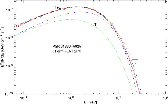
Fig. 1.
Tachyonic γ -ray spectrum of pulsar PSR J1836 + 5925. Data points from Fermi-LAT (2nd Pulsar Catalog) [10] and [26]. The solid curve T + L depicts the unpolarized tachyonic energy flux
 , cf.
(3.3) and
(5.2), obtained by adding the transversal flux component
, cf.
(3.3) and
(5.2), obtained by adding the transversal flux component
 (dotted curve, labeled T) and the longitudinal component
 (dashed curve, L). The polarization components
 are compiled in
(3.6),
(3.7) and (3.8). The dot-dashed and double-dot-dashed curves depict the upper and lower 2σ (95%) confidence limits of the
χ2 fit. The power-law ascent
(5.5) is followed by a cross-over into subexponential Weibull decay, cf.
(5.3). The spectral parameters listed in
Table 1 are similar to Geminga
[9]. The mass scaling exponent
ρ lies below 1/2, which causes a rapid spectral cutoff and renders the radiation superluminal, cf.
(4.3). The distance estimate for this pulsar is
d ≈ 0.5 ± 0.3 kpc. (5 dof,
χ2≈6.8.)
are compiled in
(3.6),
(3.7) and (3.8). The dot-dashed and double-dot-dashed curves depict the upper and lower 2σ (95%) confidence limits of the
χ2 fit. The power-law ascent
(5.5) is followed by a cross-over into subexponential Weibull decay, cf.
(5.3). The spectral parameters listed in
Table 1 are similar to Geminga
[9]. The mass scaling exponent
ρ lies below 1/2, which causes a rapid spectral cutoff and renders the radiation superluminal, cf.
(4.3). The distance estimate for this pulsar is
d ≈ 0.5 ± 0.3 kpc. (5 dof,
χ2≈6.8.)
-
-
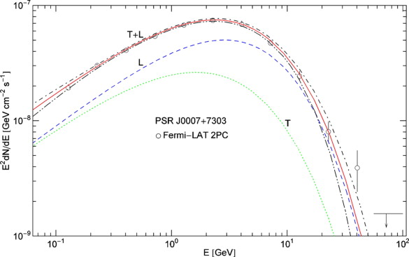
Fig. 2.
Tachyonic energy flux of pulsar PSR J0007 + 7303. Data points from Fermi-LAT [10] and [27]. The caption to Fig. 1 applies. The polarization components are labeled T and L, the ±2σ error band is indicated by the dot-dashed curves. The transversal radiation is linearly polarized and weaker than the longitudinal component. The scaling exponent ρ of the tachyon mass is about 1/2, cf. Table 1, which is just the border between sub- and superluminality, cf. (4.3). d ≈ 1.4 ± 0.3 kpc. (7 dof, χ2≈6.2.)
-
-
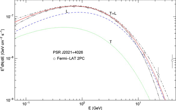
Fig. 3.
Tachyonic γ -ray spectrum of pulsar PSR J2021 + 4026. Data points from Fermi-LAT [10] and [28], the caption to Fig. 1 applies. The tachyonic mass scaling exponent ρ lies above 1/2, resulting in a gradual spectral cutoff and in subluminal γ -rays, cf. (4.3). The spectral parameters in Table 1 are similar to the Vela pulsar [9]; the spectral peak is located at about the same energy, as the larger decay exponent
 is compensated by the smaller shape parameter 1 − ρ , cf.
(5.3). (The flux amplitude
at of the pulsars discussed in
[9] corresponds to
is compensated by the smaller shape parameter 1 − ρ , cf.
(5.3). (The flux amplitude
at of the pulsars discussed in
[9] corresponds to
 , cf.
Table 1, and the decay exponent
β∞ in
[9] to
.) The pulsar distance is
d ≈ 1.5 ± 0.4 kpc. (6 dof,
χ2≈1.3.)
, cf.
Table 1, and the decay exponent
β∞ in
[9] to
.) The pulsar distance is
d ≈ 1.5 ± 0.4 kpc. (6 dof,
χ2≈1.3.)
-
-
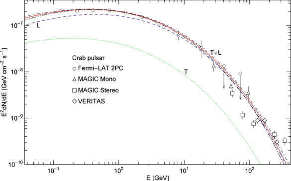
Fig. 4.
Tachyonic energy flux of the Crab pulsar PSR J0534 + 2200. Data points from Fermi-LAT [10] and [29], MAGIC [11] and [30] and VERITAS [31]. The caption to Fig. 1 applies. The emission is subluminal, the Weibull shape parameter of the spectral tail is noticeably smaller (1 − ρ ≈ 0.2) and the decay exponent
larger than of the other pulsars, cf.
Table 1.
A Weibull exponential with small shape parameter and large decay
exponent can approximate power-law decay over a finite energy range, cf.
(5.3) and
(6.2),
although the spectral tail remains slightly curved and thus
distinguishable from a power-law slope (linear in a double-logarithmic
plot). d ≈ 2.0 ± 0.5 kpc. (14 dof,
χ2≈67.)
-
Table 1.
Parameters of the tachyonic energy flux of the pulsars in Fig. 1, Fig. 2, Fig. 3 and Fig. 4. The γ -rays are radiated by a thermal plasma with electron index α = −2, cf. (3.1). The fine-structure scaling exponent σ=η∞−2ρ is inferred from the scaling exponent ρ of the tachyon mass, cf. (4.2), and from the exponent η∞ in (4.9) determining the slope of the initial power-law ascent of the flux density. The fitting parameters are η∞, ρ , the decay exponent
, cf.
(4.7), and the flux amplitude
A∞, cf.
(4.9). The spectral fits depicted in the figures are based on the differential flux density
, cf.
(3.3) and
(5.2). The Weibull shape parameter determining the subexponential decay of the spectral tails is 1 − ρ , cf.
(5.3). The indicated standard deviations are extracted from the covariance matrix of the
χ2 functional. -
σ ρ η∞ 

PSR J1836 + 5925 −0.013 0.419 ± 0.029 0.826 ± 0.045 2.10 ± 0.19 6.04±0.60×10⁻⁸ PSR J0007 + 7303 −0.259 0.504 ± 0.042 0.749 ± 0.062 1.73 ± 0.29 2.57±0.36×10⁻⁸ PSR J2021 + 4026 −0.436 0.630 ± 0.051 0.824 ± 0.183 3.93 ± 0.10 2.55±1.69×10⁻⁷ Crab pulsar −0.824 0.809 ± 0.019 0.795 ± 0.159 6.83 ± 1.45 
- Full-size table
6. Conclusion: spectral decay and the extreme quantum regime
The
basic results have been summarized in the introduction. Here, we
conclude with some remarks on Weibull decay of spectral tails,
polarization and the quantum limit. We have not discussed the extreme
quantum limit of the flux densities
(3.6),
(3.7) and (3.8) (realized by large tachyon–electron mass ratios
![]() , cf.
(3.4)) in any detail, as the spectral fits in
Fig. 1,
Fig. 2,
Fig. 3 and Fig. 4 are performed in the quasiclassical regime.
, cf.
(3.4)) in any detail, as the spectral fits in
Fig. 1,
Fig. 2,
Fig. 3 and Fig. 4 are performed in the quasiclassical regime.
6.1. Sub- and superexponential decay of spectral tails
The second-quantized flux densities
(3.6),
(3.7) and (3.8) decay for large electronic Lorentz factors, since
(βγ)α+2Γ(−α−1,βγ)∼e−βγ. The minimal transversal/longitudinal Lorentz factor
![]() in
(2.14) increases at least linearly with
ω , so that the ultimate decay of the flux densities is exponential or superexponential for
ω→∞. In contrast, if
ω varies in a finite interval (defined by data sets) and the tachyonic mass amplitude
in
(2.14) increases at least linearly with
ω , so that the ultimate decay of the flux densities is exponential or superexponential for
ω→∞. In contrast, if
ω varies in a finite interval (defined by data sets) and the tachyonic mass amplitude
![]() is sufficiently small and the electron temperature high, then the approximation
is sufficiently small and the electron temperature high, then the approximation
![]() used in
(5.1) and
(5.2) is applicable in this interval, and the decay factor
used in
(5.1) and
(5.2) is applicable in this interval, and the decay factor
![]() in the flux density
(5.3) is subexponential for
0<ρ<1 and superexponential for negative
ρ . Subexponential decay within a finite interval can be realized in the quasiclassical regime, where the mass ratios
in the flux density
(5.3) is subexponential for
0<ρ<1 and superexponential for negative
ρ . Subexponential decay within a finite interval can be realized in the quasiclassical regime, where the mass ratios
![]() defined in
(2.8) and
(3.4) are small, but also in the opposite limit, the extreme quantum regime where
defined in
(2.8) and
(3.4) are small, but also in the opposite limit, the extreme quantum regime where
![]() , see the following remark.
, see the following remark.
6.2. Spectral decay and polarization in the quantum limit
Instead of using the factorization
(3.9) designed for the quasiclassical regime, we split the minimal Lorentz factor as
![]() , where, cf.
(3.5),
, where, cf.
(3.5),

6.3. Subexponential decay approximating power-law decay in the quasiclassical regime
If the scaling exponent
ρ of the tachyon mass in
(4.2) is close to one,
0<1−ρ=ε≪1, then the Weibull exponential
![]() in the flux asymptotics
(5.3) admits the epsilon expansion
in the flux asymptotics
(5.3) admits the epsilon expansion
References
-
- [1]
-
Annu. Rev. Astron. Astrophys., 52 (2014) arXiv:1312.2913
-
- [2]
-
J. Appl. Mech., 18 (1951), p. 293
- |
-
- [3]
-
Transition Radiation and Transition Scattering
-
Hilger, Bristol (1990)
-
- [4]
-
Phys. Usp., 39 (1996), p. 973
- | |
-
- [5]
-
Phys. Usp., 45 (2002), p. 341
- | |
-
- [6]
-
Vavilov–Cherenkov and Synchrotron Radiation
-
Kluwer, Dordrecht (2004)
-
- [7]
-
Proc. R. Soc. A, Math. Phys. Eng. Sci., 462 (2006), p. 689
- |
-
- [8]
-
Phys. Lett. A, 377 (2013), p. 3247
- | | |
-
- [9]
-
Europhys. Lett., 106 (2014), p. 39001
- | |
-
- [10]
-
Astrophys. J. Suppl. Ser., 208 (2013), p. 17
-
- [11]
-
Astron. Astrophys., 540 (2012), p. A69
- | |
-
- [12]
-
Ann. Phys., 322 (2007), p. 677
- | | |
-
- [13]
-
Europhys. Lett., 102 (2013), p. 61002
- | |
-
- [14]
-
Sov. Phys. Dokl., 5 (1961), p. 782
-
- [15]
-
Europhys. Lett., 16 (1991), p. 121
- |
-
- [16]
-
Phys. Scr. T, 2A (1982), p. 182
-
- [17]
-
Eur. Phys. J. C, 49 (2007), p. 815
- | |
-
- [18]
-
Physica A, 320 (2003), p. 329
- | | |
-
- [19]
-
J. Phys. A, Math. Gen., 38 (2005), p. 2201
- | |
-
- [20]
-
Eur. Phys. J. D, 32 (2005), p. 241
- | |
-
- [21]
-
Mater. Today, 14 (2011), p. 34
- | | | |
-
- [22]
-
Physica A, 387 (2008), p. 3480
- | | |
-
- [23]
-
Physica B, 405 (2010), p. 1022
- | | |
-
- [24]
-
Europhys. Lett., 104 (2013), p. 19001
- | |
-
- [25]
-
Physica A, 394 (2014), p. 110
- | | |
-
- [26]
-
Astrophys. J., 712 (2010), p. 1209
- | |
-
- [27]
-
Astrophys. J., 744 (2012), p. 146
- | |
-
- [28]
-
Astrophys. J., 700 (2009), p. 1059
- | |
-
- [29]
-
Astrophys. J., 708 (2010), p. 1254
- | |
-
- [30]
-
Astrophys. J., 742 (2011), p. 43
- | |
-
- [31]
-
Science, 334 (2011), p. 69
- |
-
- [32]
-
Eur. Phys. J. C, 69 (2010), p. 241
- | |
-
- [33]
-
Europhys. Lett., 89 (2010), p. 39002
- | |
-
- [34]
-
Physica A, 307 (2002), p. 375
- | | |
-
- [35]
-
Opt. Commun., 282 (2009), p. 1710
- | | |
-
- [36]
-
Phys. Lett. A, 377 (2013), p. 945
- | | |
-
- [37]
-
Appl. Math. Comput., 225 (2013), p. 228
- | | |
Copyright © 2014 Elsevier B.V. All rights reserved.


