Tachyonic Cherenkov densities of an ultra-relativistic electron plasma.
•
Subexponential spectral decay of the GeV/TeV γ-ray flux of supernova remnants.
•
Cherenkov fits to the γ-ray spectra of the Crab Nebula, SNR IC 443 and SNR W44.
•
Dispersive Maxwell–Proca radiation fields with frequency-dependent tachyon mass.
•
Transversal/longitudinal radiation densities & polarization degree of the γ-ray flux.
Abstract
The subexponential decay observed in the γ-ray spectral maps of supernova remnants is explained in terms of tachyonic Cherenkov emission from a relativistic electron population. The tachyonic radiation densities of an electronic spinor current are derived, the total density as well as the transversal and longitudinal polarization components, taking account of electron recoil. Tachyonic flux quantization subject to dispersive and dissipative permeabilities is discussed, the matrix elements of the transversal and longitudinal Poynting vectors of the Maxwell–Proca field are obtained, Cherenkov emission angles and radiation conditions are derived. The spectral energy flux of an ultra-relativistic electron plasma is calculated, a tachyonic Cherenkov fit to the high-energy (1 GeV to 30 TeV) γ-ray spectrum of the Crab Nebula is performed, and estimates of the linear polarization degree are given. The spectral tail shows subexponential Weibull decay, which can be modeled with a frequency-dependent tachyon mass in the dispersion relations. Tachyonic flux densities interpolate between exponential and power-law spectral decay, which is further illustrated by Cherenkov fits to the γ-ray spectra of the supernova remnants IC 443 and W44. Subexponential spectral decay is manifested in double-logarithmic spectral maps as curved Weibull or straight power-law slope.
Keywords
Tachyonic γ-ray spectra of supernova remnants;
Crab Nebula, SNR IC 443, SNR W44;
Subexponential Weibull spectral decay;
Maxwell–Proca radiation fields;
Quantized tachyonic Cherenkov densities;
Transversal and longitudinal polarization
1. Introduction
We attempt a tachyonic Cherenkov interpretation of the high-energy GeV–TeV spectral peak of the Crab Nebula and of supernova remnants (SNRs) in general. There are currently an electromagnetic and a hadronic radiation mechanism in vogue to model the γ-ray spectra of SNRs, namely inverse Compton scattering and pion decay ( Bühler and Blandford, 2014, Abdo et al., 2010 and Ackermann et al., 2013). If the spectral tail of the remnant is curved, one uses an inverse-Compton fit resulting in exponential decay, whereas a power-law slope is viewed as evidence for pion decay and high-energy protons producing pions in collisions with heavier nuclei. Tachyonic Cherenkov spectra allow for a unified treatment, as they can interpolate between exponential and power-law spectral tails ( Tomaschitz, 2014), due to the frequency-dependent tachyon mass manifested by a subexponential decay factor in the energy flux.
We derive the quantized tachyonic Cherenkov densities generated by a freely propagating electron current in a permeable spacetime, the total radiation density as well as its transversal and longitudinal components. We average these densities over a relativistic electron plasma, calculate the spectral energy flux, and perform tachyonic Cherenkov fits to the high-energy spectrum of the Crab Nebula (Bühler and Blandford, 2014, Abdo et al., 2010, Aharonian et al., 2006, Abramowski et al., 2014 and Buehler et al., 2012) and the SNRs IC 443 and W44 (Ackermann et al., 2013, Albert et al., 2007, Acciari et al., 2009 and Giuliani et al., 2011). The frequency variation of the tachyon mass determines the decay of the energy flux, which is subexponential Weibull decay in the case of the Crab Nebula and a power-law slope for SNR IC 443 and SNR W44, even though the electron distributions are exponentially cut by their Boltzmann factor. The aim is to derive explicit formulas for the tachyonic radiation densities and put them to test by performing spectral fits to these remnants.
In Section 2, we outline the formalism of Maxwell–Proca radiation fields with negative mass-square in a dispersive and dissipative spacetime defined by complex frequency-dependent permeabilities. In Section 3, we discuss tachyonic flux quantization, starting with the discrete power coefficients of a free quantum current, and derive the matrix elements of the energy flux vectors by applying box quantization. In Section 4, we perform the continuum limit of the discrete power coefficients, obtaining in this way the quantized tachyonic Cherenkov densities. For each radiation frequency, there is a minimal Lorentz factor of the radiating charge which has to be exceeded for Cherenkov emission to occur at this frequency, and we explain how the emission angles of transversal and longitudinal quanta are related to this radiation condition.
In Section 5, we specialize the radiation densities to radiation from freely moving electrons, using the matrix elements of a Dirac current as radiation source. We derive the transversal and longitudinal radiation densities, which can be done quite explicitly without the need to specify the frequency dependence of the dispersive and absorptive permeabilities and the tachyon mass. The spectral densities are given in electronic energy/velocity parametrization as well as in Lorentz representation.
In Section 6, we average the tachyonic radiation densities over a relativistic electron distribution to model the spectral energy flux of supernova remnants. The GeV and TeV flux of the remnants depends on two decay factors. One is due to energy dissipation, the exponential being determined by the imaginary part of the wavenumbers defined by the complex dispersion relations. The second decay factor is a combination of the Boltzmann weight of the radiating electron population and the frequency-dependent tachyon mass and results in subexponential Weibull or power-law spectral decay of the flux densities. We calculate the transversal and longitudinal flux components and discuss their semiclassical and quantum limits and the effect of the longitudinal radiation on the transversal linear polarization degree. Fig. 1, Fig. 2 and Fig. 3 depict tachyonic Cherenkov fits to the γ-ray spectra of the Crab Nebula and the remnants IC 443 and W44, which admit subexponential spectral tails stretching over an extended energy range. In Section 7, we present our conclusions.
Fig. 1.
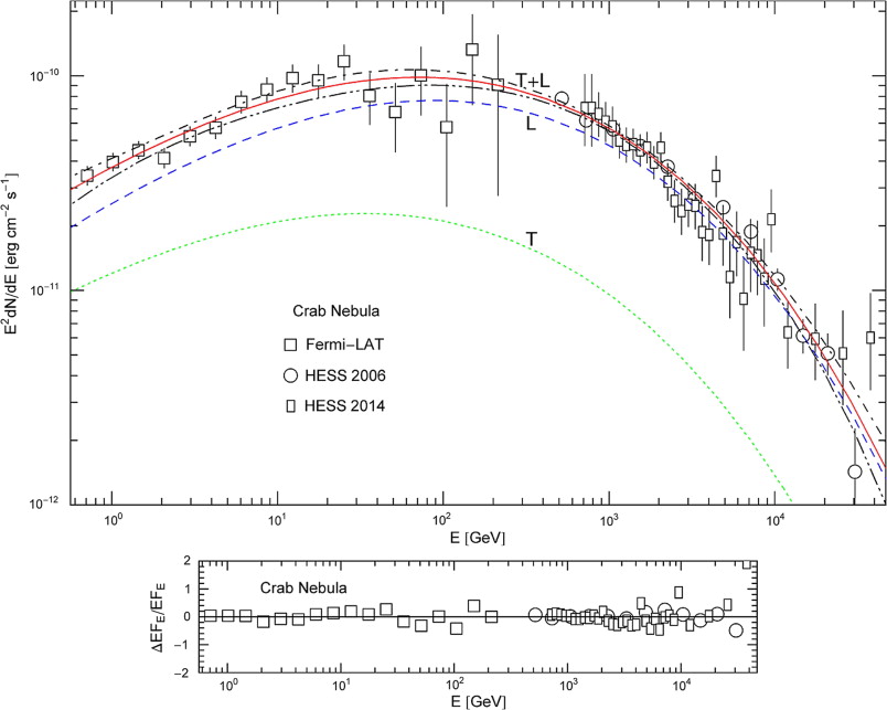
GeV to TeV γ-ray flux of the Crab Nebula (d ≈ 2 kpc). Data points from Fermi-LAT ( Buehler et al., 2012) and HESS ( Aharonian et al., 2006 and Abramowski et al., 2014). The solid curve T + L depicts the total tachyonic energy flux , cf. (6.9), obtained by adding the transversal flux component (dotted curve, labeled T) to the longitudinal flux (dashed curve, L). The transversal radiation is linearly polarized, cf. (6.10). The error band defined by the dot-dashed curves indicates the upper and lower 2σ (95%) confidence limits of the least-squares fit (57 dof, χ2≈62.5). The fine-structure scaling exponent σ = η − 2ρ ≈ −1.01 is inferred from the scaling exponent of the tachyon mass, ρ = 0.843 ± 0.029, and from the exponent η = 0.680 ± 0.19 determining the slope of the initial power-law ascent of the energy flux. The fitting parameters are η, ρ , the decay exponent and the flux amplitude . The residuals are depicted in the lower panel.
High-energy flux of SNR IC 443 (d ≈ 1.5 kpc). Data points from Fermi-LAT ( Ackermann et al., 2013), VERITAS ( Acciari et al., 2009) and MAGIC ( Albert et al., 2007). The caption to Fig. 1 applies, the fit T + L is performed with the total flux (6.12). The parameters extracted from the least-squares fit (28 dof, χ2≈24.9) are η ≈ 1.83 (slope of the initial power-law ascent), κ ≈ 1.46 (slope of the power-law decay), (decay exponent depending on electron temperature and tachyonic mass amplitude), μ[GeV−ρ]≈1.41 (defining the cross-over energy scale μ−1/ρ[GeV]≈0.35) and (flux amplitude), cf. Section 6.2.2. The fine-structure scaling exponent σ ≈ 0.49 and the scaling exponent of the tachyon mass ρ ≈ 0.33 are inferred from η, κ and , cf. (6.14). The asymptotic low- and high-frequency flux limits (6.13) are power laws appearing linear in this double-logarithmic plot (dot-dashed and double-dot-dashed lines).
Tachyonic γ-ray flux of SNR W44 (d ≈ 2.9 kpc). Data points from Fermi-LAT ( Ackermann et al., 2013) and AGILE ( Giuliani et al., 2011). The caption to Fig. 2 applies. The least-squares fit (20 dof, χ2≈11.5) of the energy flux (6.12) is depicted as solid curve T + L. The fitting parameters are η ≈ 2.69, κ ≈ 2.07, , μ[GeV−ρ]≈1.79 and , see the discussion after (6.14). The transversal and longitudinal flux components are labeled T and L; the longitudinal flux is by almost one order of magnitude higher than the transversal component. The fine-structure scaling exponent σ ≈ 1.69 and the scaling exponent of the tachyon mass ρ ≈ 0.50 are obtained from the scaling relations (6.14). The dot-dashed and double-dot-dashed straight lines show the asymptotic flux limits (6.13). The cross-over energy scale is μ−1/ρ[GeV]≈0.31. The flux points lie in the cross-over region.
subject to the constitutive relations , and , . The field strengths and are related to the vector potential by , . These relations define the inductions , and the inductive potential . The Fourier time-transform reads with reality condition . The complex permeabilities (ε0(ω),μ0(ω)) and (ε(ω),μ(ω)) have a positive real part and satisfy ε⁎(ω)=ε(−ω), and the same reality condition holds for the complex frequency-dependent tachyon mass, . Current conservation, , implies the Lorentz condition . The subscript Ω of the current refers to a frequency-dependent coupling constant, , , with reality condition Ω⁎(ω)=Ω(−ω) on the scale factor. As the external current is conserved, so is the dressed current . A manifestly covariant version of the foregoing can be found in Tomaschitz, 2014a and Tomaschitz, 2014b.
The transversal and longitudinal components of the vector potential satisfy and , respectively, and analogously for the current. The time-separated wave equations read with λT=μ and λL=ε0μ0/ε, where denote the dispersion relations (Tomaschitz, 2013)
The transversal/longitudinal components of are identified by means of the Lorentz condition, , , and the corresponding charge densities via current conservation, , , which gives the wave equation . Wave solutions are found as , with Green function (Ginzburg, 1996 and Ginzburg, 2002; Afanasiev et al., 1999; Afanasiev and Shilov, 2000) and wavenumbers kT,L=sign(κT,L,Im)κT,L. The tachyonic wavenumbers satisfy , in contrast to the above reality condition. In dipole approximation,
projected onto a triad of orthonormal polarization vectors, , . Here, n=x/r is the longitudinal polarization vector of the outgoing spherical wave, coinciding with the unit wave vector. As for the polarization triad, we use two real transversal vectors ε1,2, so that ε1, ε2 and n constitute a right-handed triad. We use the coordinate unit vector e3 as polar axis, ne3=cosθ, choose ε1 orthogonal to n and e3, and place ε2 into the plane generated by n and e3,
so that n=ε1×ε2 cyclically. Occasionally, we will write ε3 for n. As for the angular parametrization, we use x=rsinθcosφ, y=rsinθsinφ, z=rcosθ, to find
The e1,2,3 are Cartesian coordinate unit vectors. Instead of the transversal projections onto real linear polarization vectors, we can use with a complex pair of circular polarization vectors.
We find the asymptotic polarized components of the vector potential as, cf. (2.4),
We start with the current matrix element and apply the truncated Fourier transform , cf. (2.10). The subscripts m and n label the initial and final electron state, ωm and ωn are the corresponding electron energies, and ωmn=ωm−ωn is the frequency of the emitted tachyon. We will use the limit definitions and of the delta function, δ(1,2),T→∞(ω)=δ(ω). We thus find
where kT,L,Re(−ω)=−kT,L,Re(ω). Here, kT,L,Re(ω) is the real part of the tachyonic wavenumber, positive for positive frequencies. The same relation (3.2) holds for and , so that we can replace and in (3.1). Using an orthonormal triad of polarization vectors, cf. (2.5) and (2.6), we define , and analogously with , so that we can also replace , in (3.1). The squared matrix elements can thus be written as
where we have put ωmn=ω, which is the frequency of the tachyon radiated in the transition. The radiant power in the respective polarization is obtained by integrating the flux through a sphere of radius r→∞, , where dΩ=sinθdθdφ is the solid-angle element:
where km and kn are the initial and final electron momenta, and kmn=km−kn and ω=ωmn denote momentum and energy of the emitted tachyon. The domain of integration L3 refers to box quantization, see after (4.1). We use the limit definitions (2π)3δ(1)(k;L)=∫L3eikxd3x and of the 3D delta function, δ(1,2)(k;L→∞)=δ(k), to obtain
where we use box quantization, that is, periodic boundary conditions on a box of size L3 for the wave functions ∝exp(iknx) defining the free electron current. Thus, kn=2πmn/L, and the summation in (4.1) is over integer lattice points mn. We introduce polar coordinates for kn with km as polar axis, kmkn=knkmcosθ, replace d3kn by and integrate over the polar angle,
symmetric with respect to the interchanges km↔kn and kn↔kT,L,Re. The electronic dispersion relations are and for the initial and final state. The tachyonic wavenumbers kT,L,Re(ω) are stated after (2.2), and ω=ωmn is the energy of the radiated tachyon. By assembling (3.10), (4.1) and (4.2), we find the differential power coefficients
The total power transversally/longitudinally radiated is . To identify the spectral densities, we introduce ω=ωmn=ωm−ωn as integration variable, ωndωmn=−kndkn, pT(i),L(ω)dω=−dPT(i),L(ωmn), so that . The upper integration boundary ωm is the frequency of the initial electron state. The spectral densities pT(i),L(ω) can be read off from (4.4),
and of the electronic dispersion relations, cf. after (4.3), and performed a summation over the spins of the final electron state. kT,L(ω)n (with n=x/r) is the wave vector of the outgoing spherical waves, and kT,L,Re(ω) is the real part of the tachyonic wavenumber, cf. after (2.2). There are two transversal polarization components, in contrast to a classical current ( Tomaschitz, 2014b) where the projection vanishes. In Section 5, we will give explicit formulas for the radiation densities, based on the general radiation densities (4.5) and the projections (4.6) of a free relativistic spinor current onto the polarization vectors.
4.2. Radiation conditions
The argument in the Heaviside function in (4.3) factorizes as
We write ω for the energy ωmn=ωm−ωn of the emitted tachyon and E for ωm, so that ωn=E−ω. Thus, the electronic dispersion relations stated after (4.3) read km=υE and
Since E≥ω, the first factor is positive. The step function in the spectral densities (4.5) can thus be replaced by , where is the second factor in (4.10) divided by 2E,
The positive zero of determines the γ range in which a frequency ω can be radiated.
If the imaginary parts of the permeabilities and the tachyon mass are much smaller than their real parts, we can expand the dispersion relations (2.2) in the imaginary parts to find in leading order , where denote the generalized real mass-squares
with . The leading order of the imaginary part kT,L,Im of the tachyonic wavenumber in the exponential damping factor of the spectral densities (4.5) is linear in the imaginary parts of the permeabilities (Tomaschitz, 2014a). Substituting into (4.12), we find the positive zero of as
with the shortcuts and . The electron must have a Lorentz factor exceeding to radiate at ω , and the mass-squares must be positive for to be positive.
4.3. Transversal and longitudinal Cherenkov angles
The electronic wave vectors of the initial and final state are km=k0,mkm and kn=k0,nkn, cf. after (4.3). We place these vectors into the (x,z) plane and identify km with the polar z axis. The electronic/tachyonic unit wave vectors can then be parametrized as k0,m=(0,0,1), k0,n=(sinθn,0,cosθn) and n=(sinθ,0,cosθ). Energy–momentum conservation (4.7) gives
Since E=ω+ωn, this is positive, 0≤θ<π/2, the radiation being emitted into a forward cone, k0,mn=cosθ, where θ is the angle between the tachyonic wave vector and the momentum of the radiating electron. We will write θT,L for θ , as the Cherenkov angles differ for transversal and longitudinal emission. Inequality cosθT,L≤1 is thus equivalent to the radiation condition , cf. (4.11). In (4.16), we substitute , cf. (4.13), and note dcosθT,L/dE<0, so that θT,L increases with increasing electron energy, the maximal angle being . The electromagnetic emission angle is recovered with .
5. Tachyonic Cherenkov densities of spinning charges
5.1. Polarized radiation densities
The Cherenkov densities of a spinor current are assembled by substituting the squared polarized current matrices (4.6) into the spectral densities (4.5). The transversal densities are
We have renamed the radial variable in the exponential as d (distance of the detector from the radiation source). The longitudinal radiation density reads
In the exponential, we expand kT,L,Im in the imaginary parts of the permeabilities, retaining only the leading order linear in the imaginary parts. All other terms in (5.1) and (5.2) only depend quadratically on the imaginary parts of the permeabilities. Thus we can approximate , and , . To remove the subscript indices m and n in the spectral densities, we write ω=ωmn, ωm=E, ωn=E−ω, use the parametrization (4.9) of the electronic wavenumbers km, kn and replace the argument in the step function by in (4.11). Hence, cf. (5.1),
where E and denote energy and speed of the radiating electron. Finally we replace the squared tachyonic wavenumbers by substituting , where are the generalized mass-squares (4.13). The total transversal density pT=pT(1)+pT(2) is obtained by replacing the ratio ω2/(4E2) in pT(2) by . The electromagnetic limit ( Afanasiev et al., 2006) of pT(ω) is recovered by putting the tachyon mass in the generalized mass-squares (4.13) to zero and by substituting and into (5.3).
5.2. Spectral densities of a free Dirac current in Lorentz parametrization
We parametrize the spectral densities (5.3) and (5.4) by electron mass and Lorentz factor, substituting E=mγ and . The transversal densities then read
with in (4.12). The total transversal density pT(ω,γ)=pT(1)+pT(2) is obtained by replacing the factor () in pT(2) by (). In the longitudinal density (5.4), we replace by , cf. after (4.13):
The classical tachyonic Cherenkov densities (Tomaschitz, 2014b) are recovered by performing the limit m→∞ in the quantum densities (5.5) and (5.6), so that the electron mass drops out; density pT(1)(ω,γ) vanishes in this limit.
6. Tachyonic flux densities of a relativistic electron plasma
6.1. Tachyonic energy flux
We average the tachyonic Cherenkov densities (5.5) and (5.6) over a relativistic thermal electron distribution, , parametrized with the electronic Lorentz factor γ ( Tomaschitz, 2014c). Aβ is the normalization constant, β=m/(kBT) the temperature parameter and m the electron mass. The differential energy flux and number flux dNT(i),L/dω read ( Tomaschitz, 2010 and Tomaschitz, 2010a)
where 〈pT(i),L〉 are the averaged transversal/longitudinal Cherenkov densities, d is the distance to the source, and the minimal electronic Lorentz factor (4.14). The total energy flux employed in the spectral fits is obtained by adding the three polarization components. The transversal flux components read explicitly
The flux amplitude is at=αt0Aβ/(4πd2β3), with αt0=q2/(4π), and for γ we have to substitute or in (4.14). The transversal/longitudinal mass-squares MT,L are stated in (4.13), and we use the shortcuts and as in (4.14). The total transversal energy flux is obtained by replacing the factor () in by (). The semiclassical regime is attained for , the classical limit being , and the quantum regime is realized in the opposite limit, for .
6.2. Semiclassical regime
In the semiclassical regime , it is convenient to factorize the minimal Lorentz factor as , where, cf. (4.14),
This limit is effectively uniform, even though the parameter xT,L can become large (depending on ), because of the exponential cutoff. The quantum limit discussed in Section 6.3 is uniform as well for the same reason.
In the case of coinciding transversal/longitudinal attenuation factors (which happens if kT,Im=kL,Im or if the imaginary parts of the wavenumbers are small enough for the absorption to become negligible) and permeabilities satisfying ε0,Reμ0,Re=1, εReμRe=1, we can drop the subscripts T,L. (kT,Im=kL,Im requires εIm/εRe+μIm/μRe to coincide with ε0,Im/ε0,Re+μ0,Im/μ0,Re; explicit formulas for the wavenumbers kT,L linearized in the imaginary parts of the permeabilities are given in Tomaschitz (2014a).) The mass-squares in (4.13) then simplify to with , so that and , and we can add the classical flux limits (6.7) to find the total flux
where , cf. (6.4), valid in the classical regime .
6.2.1. Subexponential Weibull decay of the flux densities: γ-ray spectral fit to the Crab Nebula
We rescale the tachyonic fine-structure constant , αt0=q2/(4π), with the magnetic permeability, , and specify the frequency dependence of and the rescaled tachyon mass as power laws: and . In flux densities (6.7) and (6.8), we can then replace , where . In a high-frequency interval where the energy of the radiated quanta is much larger than the tachyon mass, , we approximate , , cf. after (6.8). We thus find, cf. (6.7),
with scaling exponent η=σ+2ρ, and the polarization component vanishes in this limit. Fig. 1 shows a fit of the high-energy spectrum of the Crab Nebula based on the total flux in (6.9). The fitting parameters are recorded in the figure caption. (In the figures, we write E for ω, using GeV units.) The power-law exponent ρ of the tachyon mass can accurately be extracted from the fit. The decay is substantially weaker than exponential, but decidedly different from a straight power-law slope, appearing moderately curved in the double-logarithmic spectral plot. We assume the absorption to be negligible on Galactic length scales of a few kiloparsecs and drop the damping factor e−2kImd. (This means to use real permeabilities and a real tachyon mass, so that the dispersion relations (2.2) are real.) The second exponential in (6.9) generates subexponential Weibull decay for 0<ρ<1 ( Tomaschitz, 2014b).
In a high-temperature regime defined by , the transversal and longitudinal radiation components have comparable intensity, . At low temperature, , the longitudinal radiation overpowers the transversal component, . As there is only one transversal polarization component, we find the transversal polarization degree as
In the quantum regime, the flux component does not vanish, see Section 6.3, and we have to employ Stokes parameters to define the linear polarization degree, cf. (6.20). In the case of the Crab Nebula, we find , with ω in GeV units, cf. the caption to Fig. 1, so that ΠT[1 GeV]≈0.32 and ΠT[1 TeV]≈0.17, which means linear polarization degrees of 32% and 17% at the indicated energies.
Polarization measurements of the Crab Nebula have not been performed so far above the keV interval (Chauvin et al., 2013, Dean et al., 2008, Forot et al., 2008, Krawczynski, 2012, Chang et al., 2014 and Kislat et al., 2015). Chauvin et al. (2013) estimated a polarization degree of 28±6% in the 130–440 keV band for the total emission. In the 130–650 keV range, they found 32±7% and in the 130–1000 keV interval 34±8% linear polarization. The above estimate at 1 GeV suggests that the polarization does not substantially change in the MeV range. Earlier measurements, also with the INTEGRAL spectrometer, found 46±10% polarization for the unpulsed emission in the 100–1000 keV band (Dean et al., 2008). In the 200–800 keV band, Forot et al. (2008) found polarization for the total emission and a lower bound of 72% for the unpulsed radiation. Inverse Compton scattering in the Klein–Nishina regime with electronic Lorentz factors exceeding 10 does not produce noticeable linear polarization (Krawczynski, 2012 and Chang et al., 2014). That is, inverse Compton scattering results in unpolarized radiation in the GeV band, in contrast to tachyonic Cherenkov radiation.
We also mention the low-frequency limit (still in the classical regime ), where we can approximate x∼β (see after (6.8)) in flux densities (6.7), which leads to power-law scaling,
At high-temperature, β≪1, the transversal and longitudinal components coincide, . At low temperature, the longitudinal radiation has higher intensity, . There are no restrictions on the frequency and the temperature parameter in (6.9) and (6.11) other than the quoted inequalities.
6.2.2. Power-law decay of the spectral tails of SNR IC 443 and SNR W44
We start with the classical flux limit (6.8), rescale the tachyonic fine-structure constant, , and specify the frequency scaling of as power law like in Section 6.2.1. For the rescaled tachyon mass , we assume a linear frequency dependence subject to logarithmic correction, , with positive exponent ρ and cross-over amplitude μ. In the unpolarized flux (6.8), we substitute and approximate , , applicable for . (This condition can be met in any frequency range if the tachyonic mass scaling amplitude is sufficiently small.) Flux density (6.8) then reads
with amplitude (since in (6.8)). The longitudinal flux component is obtained by replacing the two factors of 4 by 2, cf. (6.7). The asymptotic low- and high-frequency limits of (6.12) are the power laws
with exponents η=σ+2−2ρ and . The first applies in the low-frequency regime, μωρ≪1 (still with for (6.12) to apply), the second in the opposite limit, μωρ≫1. (The cross-over energy scale is thus μ−1/ρ in frequency units. Exponent η is positive since the low-energy slope is ascending, and κ is positive due to the descending high-energy slope. In view of the asymptotic power-law scaling, it is convenient to use η and κ instead of σ and ρ as fitting parameters, substituting
into flux density (6.12). In the spectral fits in Fig. 2 and Fig. 3, we neglect absorption and drop the attenuation factor e−2kImd in (6.12) and (6.13). As the exponents η, κ and ρ are positive, is restricted to . The fitting parameters (recorded in the figure captions) are the power-law exponents η and κ defining the low- and high-energy slopes (6.13), the parameters μ and determining the location and curvature of the cross-over, and the flux amplitude .
The least-squares fits in Fig. 2 and Fig. 3 are performed with flux points located in the cross-over region. If one considers as a prescribed constant rather than as fitting parameter, any will result in a fit which is virtually indistinguishable from the curves shown in the figures. This is so because the χ2 functional minimized at constant converges to an absolute minimum for . This minimum is only insignificantly lower than the χ2 values stated in the figure captions (which were obtained by minimizing the functional with fixed at the indicated value). A much larger than 10 leaves the depicted section of the fitting curves virtually unaffected, but has a significant impact on the other fitting parameters, especially on the slope indices η and κ of the asymptotic limits (6.13) which steepen with increasing . To determine from a χ2 fit requires additional flux points in the asymptotic regions, especially along the low-energy slope, to constrain the power-law exponents η and κ of the asymptotes (6.13) depicted in Fig. 2 and Fig. 3.
6.3. Flux densities in the quantum regime
In the quantum regime , we factorize the minimal Lorentz factor (4.14) as , using the rescaled variables and , see (6.4). The transversal energy flux (6.5) can then be written as
with , and . The total flux is . This applies in the limit .
We specify power-law scaling relations for the tachyon mass and tachyonic fine-structure constant as in Section 6.2.1, , , so that . In a high-frequency interval where (but still in the quantum regime ) we approximate y∼βω/(2m) in (6.18) to obtain the exponentially decaying flux densities
with amplitude AF (defined at the beginning of Section 6.2.1) and scaling exponent η=σ+2ρ, to be compared with the classical high-frequency limit in (6.9).
As there are two degrees of transversal polarization, in contrast to the semiclassical case (6.9), we employ Stokes parameters to define the linear polarization degree. The flux is obtained by averaging spectral density pT(1)(ω,γ) in (5.5) over an electron distribution as stated in (6.1), and analogously for the second polarization component and pT(2). The spectral densities pT(i) are calculated by projecting the current of the radiating charge onto the transversal polarization vectors εi, cf. (2.5) and (4.5). They constitute an orthonormal triad together with the longitudinal polarization vector, the normalized wave vector n of the outgoing spherical wave, see after (2.4). We consider a second set of transversal polarization vectors , obtained by rotating the vectors εi through an angle of π/4 around the longitudinal polarization axis n. The transversal spectral densities for radiation linearly polarized in the directions are calculated as in (4.5), employing the projected matrix elements instead of in (4.6). The can be averaged like the densities pT(i) in (6.1), and the corresponding fluxes are denoted by . The Stokes parameters are then defined as , ; the third parameter V is found in like manner, by substituting the projections into (4.5), where ε± are the complex circular polarization vectors stated after (2.6). The transversal linear polarization degree is calculated as
coinciding with (6.10) if vanishes since in this case U=0. The normalization in (6.20) is with the measured total flux . In a high-temperature regime where y∼βω/(2m)≪1, we find , cf. (6.19). That is, the transversal radiation is linearly polarized since is negligible. The transversal and longitudinal components have equal intensity in this limit. At low temperature, y∼βω/(2m)≫1, we find , which means that the longitudinal radiation vanishes and the two transversal components have equal intensity, resulting in unpolarized transversal radiation ΠT∼0.
Thus, in the quantum limit , subexponential Weibull decay (for mass-scaling exponents in the range 0<ρ<1) arises in the low-frequency regime , in contrast to the classical counterpart (6.9). As for polarization, the same reasoning as after (6.20) applies to the high- and low-temperature limits and . At high temperature, the transversal radiation is linearly polarized and has the same intensity as the longitudinal radiation. At low temperature, a second linear polarization component emerges at the expense of the longitudinal component. The two transversal components have the same intensity, so that the transversal polarization vanishes.
7. Conclusion
The tachyonic Cherenkov densities (5.5), (5.6) of an electronic spinor current have been derived in the framework of relativistic quantum mechanics, by applying a scalar Green function in space-frequency representation to the transversal/longitudinal current projections, cf. (2.3). The effect of the frequency-dependent permeabilities and tachyon mass is evident in the generalized mass-squares (4.13) which define the radiation condition (4.14) and the Cherenkov angles (4.16), and they also determine the decay factors of the transversal and longitudinal energy flux components (6.5) and (6.6). The subexponential spectral decay of the Crab Nebula is pronounced, caused by the Weibull exponential with very small shape parameter 1−ρ≈0.16, cf. Fig. 1. This decay factor in the energy flux (6.9) can reproduce the very accurately measured subexponential decay of the TeV spectral tail. The Weibull decay of the spectral tail is derived from a tachyonic radiation model based on a Maxwell–Proca field theory.
The tachyonic energy flux produced by a thermal electron plasma can decay subexponentially (with Weibull exponent 0<ρ<1 in (6.9)), whereas inverse Compton scattering or electromagnetic synchrotron and curvature radiation result in exponential cutoffs if the cross-section or radiation density is averaged over a thermal or non-thermal electron population because of the exponential Boltzmann weight factor. Also the hadronic radiation theory of pion decay requires a non-exponential proton distribution in conjunction with a geometric fitting parameter to model the observed power-law decay and the extended cross-over region between the low- and high-frequency power-law slopes of the SNRs IC 443 and W44 (Ackermann et al., 2013). In contrast to electromagnetic Cherenkov radiation, the tachyonic Cherenkov flux admits a longitudinal polarization component, cf. (6.9) and Fig. 1, Fig. 2 and Fig. 3, due to the negative mass-square of the radiation field (Tomaschitz, 2009, Tomaschitz, 2009a and Tomaschitz, 2010b). This longitudinal component also affects the transversal linear polarization degree, cf. (6.10) and (6.20), the radiation being linearly polarized even in the GeV range, in contrast to inverse Compton scattering.
The Cherenkov densities (5.3), (5.4) define the power at large distance from the radiating source, in leading order in a 1/r expansion, derived from the tachyonic radiation fields (2.3) in dipole approximation. The radiation conditions for Cherenkov emission are positivity of the generalized mass-squares in (4.13) as well as positivity of the argument in the Heaviside factor of the radiation densities, cf. (4.11) and (4.12). The condition is equivalent to cosθT,L≤1, where θT,L is the transversal/longitudinal Cherenkov angle (4.16). When calculating the tachyonic energy flux in Sections 6.2 and 6.3, we assumed permeabilities satisfying εReμRe=1, ε0,Reμ0,Re=1, so that photonic Cherenkov radiation is forbidden ( in (4.13)). Tachyonic Cherenkov radiation arises since the generalized mass-squares stay positive owing to the tachyon mass in the field equations (2.1).
The spectral decay of tachyonic Cherenkov densities averaged over a relativistic electron distribution (6.1) is determined by the frequency-dependent tachyon mass, in the semiclassical as well as quantum regime. It can vary from exponential decay, cf. (6.19), to subexponential Weibull decay, as is the case for the Crab Nebula in Fig. 1, cf. (6.9) and (6.21), to power-law decay (6.12) which shows in the spectra of the SNRs IC 443 and W44 in Fig. 2 and Fig. 3. The flux densities (6.9) and (6.12) used in the spectral fits apply if the semiclassical condition on the tachyon-electron mass ratio is met; the opposite quantum limit is studied in Section 6.3. In the case of the remnants discussed here, the frequency dependence of the tachyon mass is nearly linear at high frequencies, cf. Section 6.2 and the captions to Fig. 1, Fig. 2 and Fig. 3. Therefore, this semiclassical condition will not be satisfied at energies sufficiently above the energy ranges depicted in the figures, in which case the quantum limit applies, that is the exponentially decaying flux density (6.19). Accordingly, there is a second high-energy cross-over from Weibull decay or power-law decay to exponential decay, located outside the range of the currently available data sets.
Weaker-than-exponential spectral decay, either Weibull decay (indicated by slightly curved slopes in double-logarithmic spectral plots as in Fig. 1) or a straight power-law slope (as in Fig. 2 and Fig. 3) has also been detected in the MeV spectra of atmospheric γ-ray flashes ( Dwyer and Uman, 2014) and solar flares ( Ackermann et al., 2014 and Ajello et al., 2014), as well as in the GeV spectra of γ-ray pulsars ( Abdo et al., 2013). Subexponential Weibull and power-law spectral tails can only extend over a finite energy range, the ultimate decay is exponential. Section 6 gives an overview of the various limit cases (semiclassical and quantum, high- and low-frequency, high- and low-temperature) of the tachyonic flux densities (6.2) and (6.3). Spectral fits are performed in finite frequency intervals, and the asymptotic approximations to these densities enumerated in Section 6 hold uniformly in finite intervals. A tachyonic γ-ray spectrum consists of an ascending power-law slope, cf. (6.11) and (6.13), followed by a cross-over region whose actual extent and curvature are mainly determined by the rescaled electronic temperature parameter β. The cross-over is followed by subexponential Weibull decay (cf. (6.9) and (6.21)) or a power-law descent (6.12), terminating in exponential decay (6.19).


.png)
 , cf. (6.9), obtained by adding the transversal flux component
  (dotted curve, labeled T) to the longitudinal flux
  (dashed curve, L). The transversal radiation is linearly polarized, cf. (6.10). The error band defined by the dot-dashed curves indicates the upper and lower 2σ (95%) confidence limits of the least-squares fit (57 dof, χ2≈62.5). The fine-structure scaling exponent σ = η − 2ρ ≈ −1.01 is inferred from the scaling exponent of the tachyon mass, ρ = 0.843 ± 0.029, and from the exponent η = 0.680 ± 0.19 determining the slope of the initial power-law ascent of the energy flux. The fitting parameters are η, ρ , the decay exponent
  and the flux amplitude
  . The residuals are depicted in the lower panel.
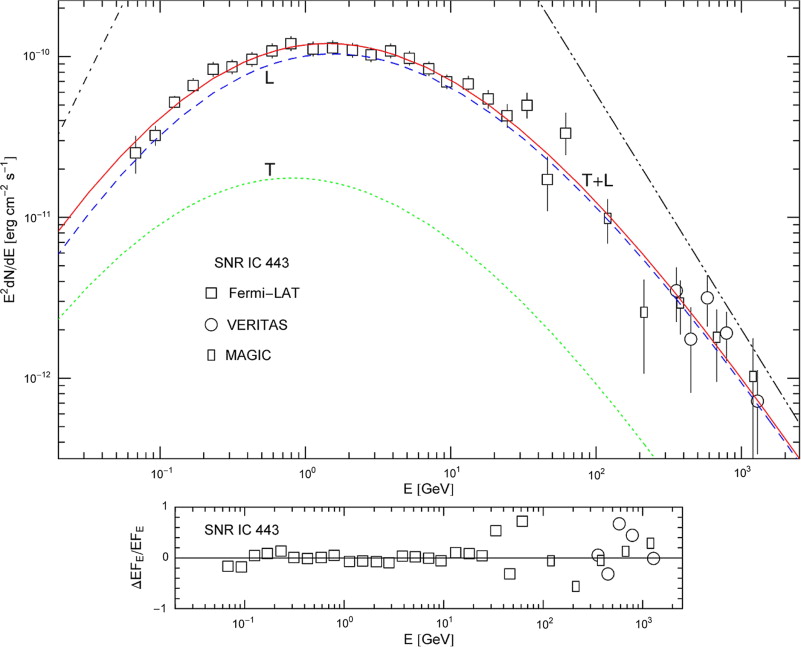
 (decay exponent depending on electron temperature and tachyonic mass amplitude), μ[GeV−ρ]≈1.41 (defining the cross-over energy scale μ−1/ρ[GeV]≈0.35) and
  (flux amplitude), cf. Section 6.2.2. The fine-structure scaling exponent σ ≈ 0.49 and the scaling exponent of the tachyon mass ρ ≈ 0.33 are inferred from η, κ and
  , cf. (6.14). The asymptotic low- and high-frequency flux limits (6.13) are power laws appearing linear in this double-logarithmic plot (dot-dashed and double-dot-dashed lines).
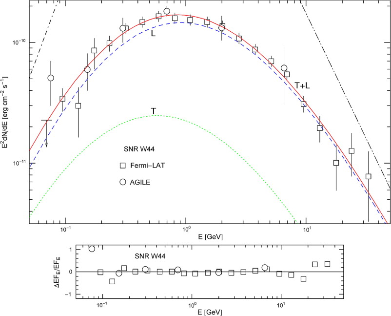
 , μ[GeV−ρ]≈1.79 and
  , see the discussion after (6.14). The transversal and longitudinal flux components are labeled T and L; the longitudinal flux is by almost one order of magnitude higher than the transversal component. The fine-structure scaling exponent σ ≈ 1.69 and the scaling exponent of the tachyon mass ρ ≈ 0.50 are obtained from the scaling relations (6.14). The dot-dashed and double-dot-dashed straight lines show the asymptotic flux limits (6.13). The cross-over energy scale is μ−1/ρ[GeV]≈0.31. The flux points lie in the cross-over region.


