
Tachyonic Cherenkov radiation in the absorptive aether


- DOI: 10.1016/j.physleta.2014.08.010
- Get rights and content
Highlights
- •
Tachyonic Maxwell–Proca radiation fields in a dispersive and dissipative spacetime.
- •
Transversal/longitudinal Poynting flux vector & associated spectral energy density.
- •
Energy dissipation quantified by absorption term in the energy conservation law.
- •
Dissipative Cherenkov densities (classical) and tachyonic attenuation lengths.
- •
Cherenkov energy flux from the shocked electron plasma of SNR RX J1713.7 − 3946.
Abstract
Dissipative tachyonic Cherenkov densities are derived and tested by performing a spectral fit to the γ-ray flux of supernova remnant (SNR) RX J1713.7 − 3946, measured over five frequency decades up to 100 TeV. The manifestly covariant formalism of tachyonic Maxwell–Proca radiation fields is developed in the spacetime aether, starting with the complex Lagrangian coupled to dispersive and dissipative permeability tensors. The spectral energy and flux densities of the radiation field are extracted by time averaging, the energy conservation law is derived, and the energy dissipation caused by the complex frequency-dependent permeabilities of the aether is quantified. The tachyonic mass-square in the field equations gives rise to transversally/longitudinally propagating flux components, with differing attenuation lengths determined by the imaginary part of the transversal/longitudinal dispersion relation. The spectral fit is performed with the classical tachyonic Cherenkov flux radiated by the shell-shocked electron plasma of SNR RX J1713.7 − 3946, exhibiting subexponential spectral decay.
Keywords
- Tachyonic radiation fields;
- Complex permeability tensors and tachyon mass;
- Energy dissipation in a permeable spacetime;
- Green functions of dispersive Maxwell–Proca fields;
- Dissipative Cherenkov flux densities;
- Shock-heated plasma of supernova remnants
1. Introduction
Decay is inherent in all composite matter, and the spacetime structure employed in physical modeling should reflect this fact. Here, we consider tachyonic wave propagation in a dissipative spacetime, the physical manifestation of the all-pervading aether. The aim is to quantify the effect of absorption on the spectral decay of radiation densities, to develop the general formalism and work out a specific example, dissipative tachyonic Cherenkov radiation [1], [2], [3], [4], [5], [6], [7], [8] and [9], and to probe the decaying energy flux by performing a spectral fit to the γ-ray emission from an ultra-relativistic plasma. For the latter, we consider the shock-heated electron population of a supernova remnant.
To this end, we start with the complex Lagrangian of a Maxwell–Proca field coupled to dissipative permeability tensors, manifestly covariantly in a frequency-space representation. In contrast to non-dissipative real permeabilities, the complex dispersion relations unambiguously determine the retarded/advanced Green function without epsilon regularization. We derive the energy conservation law for the dissipating radiation field, and identify the spectral densities of field energy and Poynting vector by time averaging. In this way, we can also quantify the energy absorption induced by the complex permeabilities and the complex tachyonic mass-square in the field equations. The attenuation lengths defining the damping factor in the classical tachyonic Cherenkov densities differ for transversal and longitudinal radiation. We average these densities over a relativistic electron gas and put them to test by performing a spectral fit to the supernova remnant RX J1713.7 − 3946, whose γ-ray flux has been measured by the Fermi satellite [10] and the ground-based atmospheric imaging array HESS [11] and [12]. The spectral fit covers five frequency decades, the GeV range up to 100 TeV.
In Section 2, we introduce the tachyonic Maxwell–Proca Lagrangian in the absorptive spacetime aether described by complex frequency-dependent permeability tensors. We explain the meaning of the complex Lagrangian and the manifestly covariant action functional, and derive the field equations and the constitutive relations, manifestly covariantly and also in 3D. In Section 3, we derive the continuity equation for the field energy in the aether defined by homogeneous and isotropic permeabilities, and extract the spectral energy flux by time averaging. In Section 4, we separate the transversal and longitudinal components of the tachyonic radiation field to obtain explicit formulas for the dissipating transversal/longitudinal energy and flux densities.
In Section 5, we derive the dispersion relations from the wave equations for the transversal and longitudinal vector potentials, as well as asymptotic formulas for the complex transversal/longitudinal wavenumbers by ascending series expansion in the imaginary parts of the permeabilities. In Section 6, we discuss spherical wave propagation in the aether, employing transversal/longitudinal Green functions in space-frequency representation. In contrast to a non-absorptive spacetime, the Green function, retarded or advanced, is already determined by the imaginary part of the dispersion relation, without the use of epsilon regularization of pole singularities prescribing residual integration paths. We use the retarded Green function in dipole approximation to obtain the attenuated radiation fields at large distance from the localized source.
In Section 7, we calculate the classical tachyonic Cherenkov densities of an inertial subluminal charge in the dissipative aether. There are two different ways to derive the Cherenkov effect. In Fermi's approach, one considers the radiating charge moving along an infinite straight line, solves the field equations in cylindrical coordinates, and calculates the flux streaming orthogonally through a cylinder around the particle trajectory [3] and [4]. A preferable method due to Tamm is to consider the trajectory within a finite time interval, so that the current distribution is compact. The time-averaged asymptotic flux through a large sphere is then calculated in dipole approximation, and the averaging period is finally extended to infinity to remove the bremsstrahlung contribution occurring at the end points of the truncated trajectory [13] and [14]. This bremsstrahlung vanishes with increasing averaging period and is not to be confused with photonic bremsstrahlung which can arise in the weakly coupled plasma of the remnant [15], [16] and [17]. The asymptotic spherical symmetry of Tamm's method is better adapted to the radiation problem studied here than an infinite cylindrical geometry. In Section 8, we average the transversal/longitudinal radiation densities over an ultra-relativistic thermal electron gas and perform a tachyonic Cherenkov fit to the γ-ray emission of SNR RX J1713.7 − 3946. In Section 9, we present our conclusions.
2. Maxwell–Proca Lagrangian in an absorptive spacetime
Throughout this article, we use a frequency-space representation of the real Proca field ![]() , suitable for dispersive and dissipative permeabilities [18], [19], [20] and [21]. Time Fourier transforms are denoted by a hat, and the reality condition is
, suitable for dispersive and dissipative permeabilities [18], [19], [20] and [21]. Time Fourier transforms are denoted by a hat, and the reality condition is ![]() . We start with the formally manifestly covariant Maxwell–Proca Lagrangian
. We start with the formally manifestly covariant Maxwell–Proca Lagrangian

We define the inductive fields ![]() and
and ![]() , as well as the dressed current
, as well as the dressed current ![]() ,
which are the manifestly covariant constitutive relations in the
absolute spacetime. Euler variation of the Lagrangian with respect to
,
which are the manifestly covariant constitutive relations in the
absolute spacetime. Euler variation of the Lagrangian with respect to ![]() gives the field equations
gives the field equations ![]() . Differentiation followed by contraction leads to the Lorentz condition
. Differentiation followed by contraction leads to the Lorentz condition ![]() , as the current is conserved. Variation of the Lagrangian with respect to
, as the current is conserved. Variation of the Lagrangian with respect to ![]() results in a different set of field equations, where the permeability
tensors and the mass-square are replaced by the conjugated quantities,
results in a different set of field equations, where the permeability
tensors and the mass-square are replaced by the conjugated quantities, ![]() ,
, ![]() .
The imaginary parts of the permeability tensors and the tachyon mass
determine whether the Green function is retarded or advanced, cf.
Sections 5.2 and 6.1.
(In contrast to real permeabilities, there are no poles on the real
axis to be circumvented by epsilon regularization, that is, by an
infinitesimal ±sign(ω)iε or ±iε insertion in the denominator of the Green function in momentum space, cf. Section 6.) For any given frequency ω , either (
.
The imaginary parts of the permeability tensors and the tachyon mass
determine whether the Green function is retarded or advanced, cf.
Sections 5.2 and 6.1.
(In contrast to real permeabilities, there are no poles on the real
axis to be circumvented by epsilon regularization, that is, by an
infinitesimal ±sign(ω)iε or ±iε insertion in the denominator of the Green function in momentum space, cf. Section 6.) For any given frequency ω , either (![]() ) or the conjugated quantities (
) or the conjugated quantities (![]() )
define retarded wave propagation, and we use the corresponding wave
equation at this frequency. For the sake of definiteness, we will
consider a frequency interval in which (
)
define retarded wave propagation, and we use the corresponding wave
equation at this frequency. For the sake of definiteness, we will
consider a frequency interval in which (![]() ) gives retarded propagation.
) gives retarded propagation.
If the permeability tensors and the tachyon mass are real and constant (frequency-independent), we can use a spacetime representation of the Lagrangian,
The 3D field strengths are ![]() and
and ![]() , and inversely
, and inversely ![]() , where εkij is the Levi-Civita 3-tensor. The 3D inductions are defined by the constitutive relations
, where εkij is the Levi-Civita 3-tensor. The 3D inductions are defined by the constitutive relations ![]() and
and ![]() , as well as
, as well as ![]() and
and ![]() for the potential, cf. after (2.2). The charge densities
for the potential, cf. after (2.2). The charge densities ![]() and
and ![]() of external and dressed current are related by
of external and dressed current are related by ![]() , and the respective 3-currents by
, and the respective 3-currents by ![]() . The 3D inhomogeneous field equations read
. The 3D inhomogeneous field equations read
The homogeneous Maxwell equations follow from the above potential representation of the field strengths, and we also mention conservation of the dressed current and the Lorentz condition,
3. Tachyonic Poynting vector and dissipative energy density
To derive the energy conservation law in an absorptive spacetime [22], [23], [24] and [25], we employ the inhomogeneous field equations (2.4), the homogeneous equations, current conservation and Lorentz condition in (2.5), as well as the constitutive relations stated before (2.4). We consider these equations at a fixed frequency ω and the conjugated equations at a different nearby frequency ω′,
We multiply the first inhomogeneous equation in (3.1) with ![]() to find
to find


In the case of constant (frequency-independent) real permeabilities and tachyon mass, the conservation law (3.6) can be stated in spacetime representation as ![]() , where [5]
, where [5]


We perform a time average of the flux vector (3.12), ![]() , to obtain
, to obtain

Since δ(1),T→∞(ω−ω′) in (3.13) converges to the delta function, we can replace ![]() by
by ![]() . Thus this calculation of the averaged flux 〈Sl〉 also applies to dissipative complex permeabilities, as we only need the limit
. Thus this calculation of the averaged flux 〈Sl〉 also applies to dissipative complex permeabilities, as we only need the limit ![]() , cf. (3.7), to perform a time average (with T→∞) of the Poynting flux vector. Analogously, we find the time-averaged energy density 〈ρ〉 by replacing
, cf. (3.7), to perform a time average (with T→∞) of the Poynting flux vector. Analogously, we find the time-averaged energy density 〈ρ〉 by replacing ![]() in (3.13) by the spectral kernel
in (3.13) by the spectral kernel ![]() in (3.8). These time averages are real, since
in (3.8). These time averages are real, since ![]() and analogously for
and analogously for ![]() , also see Section 4.
, also see Section 4.
4. Transversal and longitudinal flux and energy components
We split the vector potential and the current into a transversal and longitudinal component, ![]() with
with ![]() ,
, ![]() , and analogously the dressed current
, and analogously the dressed current ![]() , cf. Section 2, writing
, cf. Section 2, writing ![]() for
for ![]() etc. We use current conservation,
etc. We use current conservation, ![]() ,
, ![]() , cf. (2.5), to split the charge density accordingly,
, cf. (2.5), to split the charge density accordingly, ![]() ,
, ![]() . The Lorentz condition,
. The Lorentz condition, ![]() , is employed to separate the transversal and longitudinal components of the scalar potential,
, is employed to separate the transversal and longitudinal components of the scalar potential, ![]() and
and ![]() . The polarized field strengths are
. The polarized field strengths are ![]() ,
, ![]() and
and ![]() ,
, ![]() .
.
The flux vectors of the transversal and longitudinal field components read, cf. (3.7),


5. Dissipative wave equations for the tachyonic vector potential
5.1. Transversal and longitudinal dispersion relations
Substituting the potential representation of the field strengths into the inhomogeneous field equations (2.4), we find the wave equations
Transversal wave solutions of (5.3) and (5.4) are defined by the condition ![]() . The scalar component
. The scalar component ![]() follows from the Lorentz condition. A transversal solution can only exist if the current is transversal,
follows from the Lorentz condition. A transversal solution can only exist if the current is transversal, ![]() , cf. Section 4. Longitudinal wave solutions are defined by
, cf. Section 4. Longitudinal wave solutions are defined by ![]() . Applying the rotor to the vector equation (5.4), we see that longitudinal solutions can only exist if the current is longitudinal,
. Applying the rotor to the vector equation (5.4), we see that longitudinal solutions can only exist if the current is longitudinal, ![]() . Condition
. Condition ![]() implies
implies ![]() , so that Eq. (5.4) can be written as
, so that Eq. (5.4) can be written as ![]() , and
, and ![]() is obtained from the Lorentz condition,
is obtained from the Lorentz condition, ![]() .
.
5.2. Complex wavenumbers
We consider the complex squared wavenumbers ![]() in (5.2) and (5.3), where ε=εRe+iεIm, mt=mt,Re+imt,Im, etc., with positive real parts of the permeabilities and tachyon mass. We split
in (5.2) and (5.3), where ε=εRe+iεIm, mt=mt,Re+imt,Im, etc., with positive real parts of the permeabilities and tachyon mass. We split ![]() and expand in the imaginary parts of the permeabilities and mass; aT,L then contains even powers and bT,L odd ones. The transversal and longitudinal dispersion relations
and expand in the imaginary parts of the permeabilities and mass; aT,L then contains even powers and bT,L odd ones. The transversal and longitudinal dispersion relations ![]() are related by the interchange ε↔μ0, μ↔ε0. We introduce the rescaled tachyon mass
are related by the interchange ε↔μ0, μ↔ε0. We introduce the rescaled tachyon mass ![]() ,
,


6. Retarded spherical wave propagation in the spacetime aether
6.1. Reduction to scalar transversal and longitudinal Green functions
We consider the scalar Green function satisfying
The wave equations for transversal and longitudinal radiation fields read ![]() , with λT=μ and λL=ε0μ0/ε, cf. Section 5.1. The corresponding Green functions are defined by
, with λT=μ and λL=ε0μ0/ε, cf. Section 5.1. The corresponding Green functions are defined by ![]() , and wave solutions are found as
, and wave solutions are found as
6.2. Asymptotic tachyon fields
In the Green function ![]() in (6.3), we put n=x/r with r=|x| and |x′|/r≪1, and expand |x−x′|=r(1−nx′/r+⋯), to obtain the dipole approximation
in (6.3), we put n=x/r with r=|x| and |x′|/r≪1, and expand |x−x′|=r(1−nx′/r+⋯), to obtain the dipole approximation
As pointed out in Sections 4 and 5.1, the transversal fields are ![]() ,
, ![]() ,
, ![]() , and the longitudinal ones read
, and the longitudinal ones read ![]() ,
, ![]() , and
, and ![]() with
with ![]() , so that, by way of the dispersion relation in (5.3),
, so that, by way of the dispersion relation in (5.3),
The asymptotic energy flux is found by substituting these fields into Eqs. (4.1) and (4.2),
7. Dissipative tachyonic Cherenkov densities
We consider a subluminal particle x0(t) moving in the vicinity of the coordinate origin and carrying a tachyonic charge q . The charge and current densities are j0=ρ=qδ(x−x0(t)) and ![]() , so that the current transform (6.6) reads
, so that the current transform (6.6) reads

We specialize to uniform motion x0(t)=υt, where υ is the subluminal speed υ<1, and use υ as polar axis, υ=υe3, nυ=υcosθ, cf. (6.8), to obtain


In the exponential, we expand kT,L,Im
in the imaginary parts of the permeabilities, retaining only the
leading order, which is linear in the imaginary parts, cf. after (5.7). The attenuation length 1/(2kT,L,Im)
differs for transversal and longitudinal modes. All other terms in the
integrands only depend quadratically on the imaginary parts of the
permeabilities, which we neglect, ![]() ,
, ![]() . For instance, in the photonic case, we put mt=0, Ω=1, and substitute
. For instance, in the photonic case, we put mt=0, Ω=1, and substitute ![]() and
and ![]() into PT, cf. Section 5.2;
the power longitudinally radiated vanishes. The permeabilities differ
for tachyons and photons, as well as the respective fine-structure
constants, cf. after (7.8) and Ref. [19]. By means of (7.5), we identify the spectral densities determining the power
into PT, cf. Section 5.2;
the power longitudinally radiated vanishes. The permeabilities differ
for tachyons and photons, as well as the respective fine-structure
constants, cf. after (7.8) and Ref. [19]. By means of (7.5), we identify the spectral densities determining the power ![]() measured at large distance d from the source particle as
measured at large distance d from the source particle as

The constant q2/(4πħc)=αt0 in (7.6) is the tachyonic counterpart to the electric fine-structure constant e2/(4πħc)=1/137, and ![]() is the scale factor of the frequency-dependent tachyonic fine-structure constant
is the scale factor of the frequency-dependent tachyonic fine-structure constant ![]() , cf. after (2.2) and Ref. [9].
, cf. after (2.2) and Ref. [9]. ![]() can only be positive if the mass-square
can only be positive if the mass-square ![]() is positive, which is thus a radiation condition. Moreover, condition
is positive, which is thus a radiation condition. Moreover, condition ![]() has to be satisfied, where m
is the mass of the radiating charge, otherwise the classical radiation
densities have to be replaced by the quantized ones; the latter depend
on the particle mass m and converge to the classical densities in the limit m→∞, see Ref. [26] for tachyonic quantum densities (with non-absorptive real permeabilities) and their limit cases. We solve
has to be satisfied, where m
is the mass of the radiating charge, otherwise the classical radiation
densities have to be replaced by the quantized ones; the latter depend
on the particle mass m and converge to the classical densities in the limit m→∞, see Ref. [26] for tachyonic quantum densities (with non-absorptive real permeabilities) and their limit cases. We solve ![]() for γ to find the minimal Lorentz factor
for γ to find the minimal Lorentz factor ![]() for Cherenkov emission; a frequency ω can only be radiated by a charge whose Lorentz factor exceeds γT,L(ω).
for Cherenkov emission; a frequency ω can only be radiated by a charge whose Lorentz factor exceeds γT,L(ω).
8. Cherenkov spectral fit to supernova remnant RX J1713.7 − 3946
We average the tachyonic Cherenkov densities (7.6) over a relativistic thermal electron distribution, ![]() , parametrized with the electronic Lorentz factor γ . Aβ is the normalization constant, β=m/(kBT) the temperature parameter and m the electron mass. The differential energy flux
, parametrized with the electronic Lorentz factor γ . Aβ is the normalization constant, β=m/(kBT) the temperature parameter and m the electron mass. The differential energy flux ![]() and number flux dNT,L/dω read
and number flux dNT,L/dω read


We specify the permeabilities as εReμRe=ε0,Reμ0,Re=1, and put their imaginary parts to zero, so that the permeability tensors (2.2) are conformal to the Minkowski metric. The transversal/longitudinal dispersion relations in (5.2) and (5.3) are then identical, and we drop the subscripts T and L of the wavenumbers k=kRe+ikIm, which are complex because of the imaginary part of the tachyon mass, cf. Section 5.2. The minimal Lorentz factor γT,L(ω) in the flux densities (8.2) can be replaced by ![]() , since
, since ![]() , cf. (7.7). We rescale the tachyonic fine-structure constant
, cf. (7.7). We rescale the tachyonic fine-structure constant ![]() , cf. after (7.8), with the magnetic permeability,
, cf. after (7.8), with the magnetic permeability, ![]() , and specify the frequency dependence of
, and specify the frequency dependence of ![]() and the rescaled tachyon mass
and the rescaled tachyon mass ![]() in (7.7) as power laws:
in (7.7) as power laws: ![]() and
and ![]() . In the flux densities (8.2), we substitute
. In the flux densities (8.2), we substitute
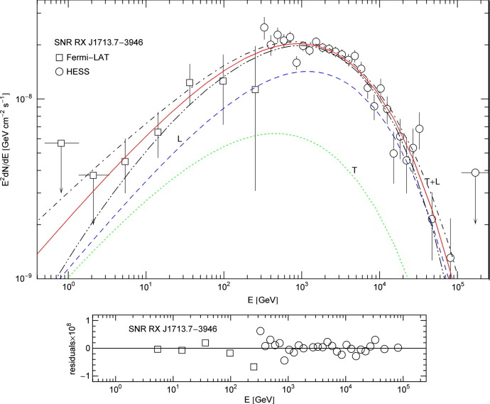
- Fig. 1.
Tachyonic γ -ray flux of supernova remnant RX J1713.7 − 3946, radiated by the shocked ultra-relativistic electron plasma. Data points from Fermi-LAT [10] and HESS [12]. The solid curve T + L depicts the unpolarized tachyonic energy flux
 , cf. (8.1) and (8.4), obtained by adding the transversal flux component
  (dotted curve, labeled T) to the longitudinal flux
  (dashed curve, L), cf. (8.2).
The transversal radiation is linearly polarized. The error band defined
by the dot-dashed curves indicates the upper and lower 1σ (68%) confidence limits of the least-squares fit (28 dof, χ2≈37.4). The fine-structure scaling exponent σ = η − 2ρ ≈ −0.98 is inferred from the scaling exponent of the tachyon mass, ρ = 0.751 ± 0.059, and from the exponent η = 0.520 ± 0.17 determining the slope of the initial power-law ascent of flux density (8.4). The fitting parameters are η , ρ , the Weibull decay exponent
(dashed curve, L), cf. (8.2).
The transversal radiation is linearly polarized. The error band defined
by the dot-dashed curves indicates the upper and lower 1σ (68%) confidence limits of the least-squares fit (28 dof, χ2≈37.4). The fine-structure scaling exponent σ = η − 2ρ ≈ −0.98 is inferred from the scaling exponent of the tachyon mass, ρ = 0.751 ± 0.059, and from the exponent η = 0.520 ± 0.17 determining the slope of the initial power-law ascent of flux density (8.4). The fitting parameters are η , ρ , the Weibull decay exponent  and the flux amplitude
  , cf. (8.4). The Weibull shape parameter determining the subexponential decay of the spectral tail is 1 − ρ ≈ 0.25. The mass scaling exponent ρ lies above 1/2, implying subluminal group velocity of the γ-rays, cf. the end of Section 8.
The imaginary part of the wavenumber in the first exponential of flux density (8.4) is ![]() , cf. after (5.7) and (6.3). The scaling relation
, cf. after (5.7) and (6.3). The scaling relation ![]() for the imaginary part of the tachyon mass (analogous to the frequency scaling of the real part, see before (8.3)) gives
for the imaginary part of the tachyon mass (analogous to the frequency scaling of the real part, see before (8.3)) gives ![]() . In the spectral fit, we assume the tachyonic attenuation length 1/(2kIm) in the considered frequency interval to be much larger than the source distance d≈1kpc and put exp(−2kImd)≈1. The second attenuation factor
. In the spectral fit, we assume the tachyonic attenuation length 1/(2kIm) in the considered frequency interval to be much larger than the source distance d≈1kpc and put exp(−2kImd)≈1. The second attenuation factor ![]() in (8.4) causes the subexponential Weibull decay [9] and [26] of the spectral tail depicted in Fig. 1. The tachyonic group velocity
in (8.4) causes the subexponential Weibull decay [9] and [26] of the spectral tail depicted in Fig. 1. The tachyonic group velocity ![]() (with
(with ![]() , cf. (5.6) and Ref. [27]) reads
, cf. (5.6) and Ref. [27]) reads ![]() , valid in the limit
, valid in the limit ![]() , which is the approximation used in flux density (8.4). In the case of SNR RX J1713.7 − 3946, the velocity of the tachyonic γ -rays is subluminal due to the scaling exponent ρ≈0.75 of the tachyon mass, see the caption to Fig. 1.
, which is the approximation used in flux density (8.4). In the case of SNR RX J1713.7 − 3946, the velocity of the tachyonic γ -rays is subluminal due to the scaling exponent ρ≈0.75 of the tachyon mass, see the caption to Fig. 1.
9. Conclusion
We
have developed a practically viable formalism to treat tachyonic
Maxwell–Proca radiation fields in the absorptive spacetime aether [28], [29], [30] and [31], in particular, to identify the spectral flux and the associated energy density. In Section 3,
we discussed the dissipating energy flux, and the stress tensor can be
dealt with analogously; to derive the conservation law for the field
momentum, one starts with the Lorentz force, ![]() , instead of
, instead of ![]() in (3.2).
Because of dispersion and energy dissipation manifested by the
absorption term in the energy conservation law, the time averaging
explained in Section 3
is necessary to extract the spectral energy and flux densities
intrinsic to the radiation field. The spacetime aether is defined by
homogeneous and isotropic permeability tensors, cf. Section 2.
Therefore, it is crucial to unambiguously identify the intrinsic field
energy subject to persistent dissipation, since it is not possible to
deal with energy by striking the balance between asymptotic fields (in-
and out-states) in non-dissipative vacuum regions, as the latter do not
exist.
in (3.2).
Because of dispersion and energy dissipation manifested by the
absorption term in the energy conservation law, the time averaging
explained in Section 3
is necessary to extract the spectral energy and flux densities
intrinsic to the radiation field. The spacetime aether is defined by
homogeneous and isotropic permeability tensors, cf. Section 2.
Therefore, it is crucial to unambiguously identify the intrinsic field
energy subject to persistent dissipation, since it is not possible to
deal with energy by striking the balance between asymptotic fields (in-
and out-states) in non-dissipative vacuum regions, as the latter do not
exist.
The complex Lagrangian (2.1) in space-frequency representation allows for a manifestly covariant formulation of the field equations and the constitutive relations, avoiding intricate time convolutions defining the inductions. In an absorptive spacetime, the complex dispersion relation rather than the choice of a residual integration path determines whether the Green function is retarded or advanced, cf. Sections 2 and 6.1. As transversal and longitudinal modes admit different dispersion relations, cf. Section 5.1, the Green functions for transversal and longitudinal propagation differ as well.
The dissipative tachyonic Cherenkov densities (7.6)
determine the power measured at large distance from the radiating
source. The radiation conditions for Cherenkov emission are the
positivity of the generalized mass-squares ![]() in the dispersion relations, cf. (7.7), and the positivity of the argument
in the dispersion relations, cf. (7.7), and the positivity of the argument ![]() in the Heaviside factor of the radiation densities (7.6). Condition
in the Heaviside factor of the radiation densities (7.6). Condition ![]() just means cosθT,L≤1, where θT,L is the transversal/longitudinal Cherenkov angle, cf. after (7.4). The effect of the real part of the tachyon mass is evident in the mass-squares
just means cosθT,L≤1, where θT,L is the transversal/longitudinal Cherenkov angle, cf. after (7.4). The effect of the real part of the tachyon mass is evident in the mass-squares ![]() , which remain positive even if the real parts of the permeabilities satisfy εReμRe=1, ε0,Reμ0,Re=1, cf. after (8.2), in which case photonic Cherenkov radiation is forbidden.
, which remain positive even if the real parts of the permeabilities satisfy εReμRe=1, ε0,Reμ0,Re=1, cf. after (8.2), in which case photonic Cherenkov radiation is forbidden.
To
highlight the difference between photonic and tachyonic Cherenkov
radiation further, we consider the transition from the classical to the
quantum regime [26]. In the spectral fit of the supernova remnant, we used the classical spectral densities (7.6). The condition for the applicability of the classical densities is a small mass ratio ![]() , where
, where ![]() are the transversal/longitudinal mass-squares (7.7) and m is the mass of the radiating electron; the quantum Cherenkov regime is realized in the opposite limit [26]. For photonic Cherenkov radiation, this condition simplifies to
are the transversal/longitudinal mass-squares (7.7) and m is the mass of the radiating electron; the quantum Cherenkov regime is realized in the opposite limit [26]. For photonic Cherenkov radiation, this condition simplifies to ![]() , as the tachyonic mass term in
, as the tachyonic mass term in ![]() vanishes, so that the energy of the radiated photons must be much
smaller than the electron mass for the classical photonic spectral
density (see after (7.5)) to apply. As pointed out after (7.8), positivity of the mass-squares
vanishes, so that the energy of the radiated photons must be much
smaller than the electron mass for the classical photonic spectral
density (see after (7.5)) to apply. As pointed out after (7.8), positivity of the mass-squares ![]() is a necessary condition for Cherenkov emission at the respective frequency, so that εReμRe>1 is required in the photonic case, a refractive index exceeding one.
is a necessary condition for Cherenkov emission at the respective frequency, so that εReμRe>1 is required in the photonic case, a refractive index exceeding one.
In contrast, a tachyonic Cherenkov density is employed in the spectral fit of the SNR shown in Fig. 1. Instead of dropping the tachyonic mass term in ![]() , we consider permeabilities satisfying εReμRe∼ε0,Reμ0,Re∼1, so that the first term in the mass-squares (7.7) vanishes. The condition
, we consider permeabilities satisfying εReμRe∼ε0,Reμ0,Re∼1, so that the first term in the mass-squares (7.7) vanishes. The condition ![]() for the classical limit then amounts to a small tachyon-electron mass ratio
for the classical limit then amounts to a small tachyon-electron mass ratio ![]() . Thus, if this mass ratio is small and the real parts of the permeabilities are close to one, the classical spectral densities (7.6) can be used to calculate the energy flux, cf. (8.1) and (8.4), even if the energy of the radiated quanta (GeV and TeV γ -rays emanating from the remnant) exceeds the electron mass, in contrast to photonic radiation which requires ω/m≪1
for the classical limit to apply. Another marked difference to photonic
Cherenkov emission is the longitudinal radiation component, which can
even overpower the transversal radiation, see Fig. 1.
The emitted tachyonic quanta can be superluminal, depending on the
scaling exponent of the tachyon mass, cf. the end of Section 8,
whereas the radiating electron gas is subluminal. Electromagnetic
radiation from superluminally rotating light spots and accelerated
superluminal particles has been studied in Refs. [32] and [33].
. Thus, if this mass ratio is small and the real parts of the permeabilities are close to one, the classical spectral densities (7.6) can be used to calculate the energy flux, cf. (8.1) and (8.4), even if the energy of the radiated quanta (GeV and TeV γ -rays emanating from the remnant) exceeds the electron mass, in contrast to photonic radiation which requires ω/m≪1
for the classical limit to apply. Another marked difference to photonic
Cherenkov emission is the longitudinal radiation component, which can
even overpower the transversal radiation, see Fig. 1.
The emitted tachyonic quanta can be superluminal, depending on the
scaling exponent of the tachyon mass, cf. the end of Section 8,
whereas the radiating electron gas is subluminal. Electromagnetic
radiation from superluminally rotating light spots and accelerated
superluminal particles has been studied in Refs. [32] and [33].
The tachyon mass in Lagrangian (2.1) is complex like the permeabilities. In the Cherenkov densities (7.6) and the averaged energy flux (8.2), the imaginary parts of the permeabilities and the tachyon mass generate the attenuation factor exp(−2kT,L,Im(ω)d), where kT,L,Im is the imaginary part of the transversal/longitudinal wavenumber and d the radial distance of the detector from the localized radiation source. At a distance of a few kiloparsecs from a Galactic source, this exponential factor is still close to one, otherwise the signal would have dissipated away. For the attenuation length 1/(2kT,L,Im) to be of the same order or larger than the source distance d, the imaginary parts of the permeabilities must be tiny. Linearization in the imaginary parts of the permeabilities and tachyon mass (starting with the dispersion relations defining the wavenumbers, cf. Section 5.2) is thus amply justified in the Cherenkov densities (7.6).
Apart
from the attenuation factor quantifying the absorption by the aether,
there emerges a second decay factor in the spectral flux densities (8.4), the Weibull exponential ![]() , where ρ is the frequency scaling exponent of the tachyon mass and
, where ρ is the frequency scaling exponent of the tachyon mass and ![]() the decay exponent inversely proportional to the temperature of the
radiating electron plasma. This decay factor results in subexponential (0<ρ<1) spectral tails as found in the γ-ray spectra of pulsars [9] and [26] and supernova remnants, cf. Fig. 1. Subexponential decay approximating power-law decay seems to be a common feature of γ-ray spectral tails and has also been detected by the AGILE satellite [34] in the MeV spectra of terrestrial γ-ray flashes [35] and [36] at thundercloud altitudes.
the decay exponent inversely proportional to the temperature of the
radiating electron plasma. This decay factor results in subexponential (0<ρ<1) spectral tails as found in the γ-ray spectra of pulsars [9] and [26] and supernova remnants, cf. Fig. 1. Subexponential decay approximating power-law decay seems to be a common feature of γ-ray spectral tails and has also been detected by the AGILE satellite [34] in the MeV spectra of terrestrial γ-ray flashes [35] and [36] at thundercloud altitudes.
References
- [1]
Phys. Usp., 39 (1996), p. 973
- | |
- [2]
Phys. Usp., 45 (2002), p. 341
- | |
- [3]
J. Phys. D, Appl. Phys., 31 (1998), p. 2760
- | |
- [4]
Physica B, 269 (1999), p. 95
- | | |
- [5]
Physica A, 307 (2002), p. 375
- | | |
- [6]
Physica A, 320 (2003), p. 329
- | | |
- [7]
Appl. Phys. B, 101 (2010), p. 143
- | |
- [8]
Phys. Lett. A, 377 (2013), p. 3247
- | | |
- [9]
Europhys. Lett., 106 (2014), p. 39001
- | |
- [10]
Astrophys. J., 734 (2011), p. 28
- [11]
Astron. Astrophys., 464 (2007), p. 235
- [12]
Astron. Astrophys., 531 (2011), p. C1
- [13]
J. Phys. D, Appl. Phys., 32 (1999), p. 2029
- | |
- [14]
J. Phys. D, Appl. Phys., 33 (2000), p. 2931
- | |
- [15]
Phys. Lett. A, 378 (2014), p. 2176
- | |
- [16]
Phys. Plasmas, 18 (2011), p. 064503
- | |
- [17]
Europhys. Lett., 91 (2010), p. 65001
- |
- [18]
Europhys. Lett., 97 (2012), p. 39003
- | |
- [19]
Phys. Lett. A, 377 (2013), p. 945
- | | |
- [20]
Europhys. Lett., 102 (2013), p. 61002
- | |
- [21]
Opt. Commun., 282 (2009), p. 1710
- | | |
- [22]
The Propagation of Electromagnetic Waves in Plasmas
(2nd ed.)Pergamon Press, Oxford (1970)
- [23]
Crystal Optics with Spatial Dispersion, and Excitons
(2nd ed.)Springer, Berlin (1984)
- [24]
Sov. Phys. JETP, 42 (1975), p. 602
- [25]
Sov. Phys. Usp., 19 (1976), p. 263
- [26]
Phys. Lett. A, 378 (2014), p. 2337
- | |
- [27]
Europhys. Lett., 98 (2012), p. 19001
- | |
- [28]
Chaos Solitons Fractals, 9 (1998), p. 1199
- | | |
- [29]
Class. Quantum Gravity, 18 (2001), p. 4395
- | |
- [30]
Physica B, 404 (2009), p. 1383
- | | |
- [31]
Eur. Phys. J. C, 69 (2010), p. 241
- | |
- [32]
Radiat. Phys. Chem., 75 (2006), p. 813
- | | |
- [33]
Europhys. Lett., 16 (1991), p. 121
- |
- [34]
Phys. Rev. Lett., 106 (2011), p. 018501
- [35]
Phys. Rep., 534 (2014), p. 147
- | | |
- [36]
J. Geophys. Res., 117 (2012), p. A05315
Copyright © 2014 Elsevier B.V. All rights reserved.


