Volume 377, Issues 45–48, 17 December 2013, Pages 3247–3253

Tachyonic Cherenkov emission from Jupiterʼs radio electrons

Roman Tomaschitz

Department of Physics, Hiroshima University, 1-3-1 Kagami-yama, Higashi-Hiroshima 739-8526, Japan

Received 29 September 2013

Accepted 11 October 2013

Available online 17 October 2013

Communicated by V.M. Agranovich

Highlights

•: Tachyonic radio emission from uniformly moving electrons in a dispersive spacetime.
•: Transversal and longitudinal flux densities due to superluminal Cherenkov effect.
•: Mildly relativistic thermal electron populations in Jupiterʼs radiation belts.
•: Spectral fit of ground-based and in-situ measurements of the Jovian radio flux.
•: Jupiterʼs low flux density at 13.8 GHz (Cassini fly-by) due to thermal spectral cutoff.

Abstract

Tachyonic Cherenkov radiation from inertial relativistic electrons in the Jovian radiation belts is studied. The tachyonic modes are coupled to a frequency-dependent permeability tensor and admit a negative mass-square, rendering them superluminal and dispersive. The superluminal radiation field can be cast into Maxwellian form, using 3D field strengths and inductions, and the spectral densities of tachyonic Cherenkov radiation are derived. The negative mass-square gives rise to a longitudinal flux component. A spectral fit to Jupiterʼs radio spectrum, inferred from ground-based observations and the Cassini 2001 fly-by, is performed with tachyonic Cherenkov flux densities averaged over a thermal electron population.

Keywords

Tachyonic Cherenkov radiation;
Superluminal radiation modes with negative mass-square;
Transversal and longitudinal tachyons;
Tachyonic Maxwell–Proca fields in a permeable spacetime;
Thermal electron plasma in Jupiterʼs radiation belts;
Cassiniʼs Jupiter fly-by and Jovian radio spectrum

1. Introduction

During the Cassini Jupiter fly-by in January 2001, an in situ measurement of the Jovian radio emission was performed, resulting in an unexpectedly low flux density of 0.44±0.15 Jy0.44±0.15Jy $0.44 \pm 0.15 Jy$ at 13.8 GHz13.8GHz $13.8 GHz$ [1], as compared to ground-based observations at 8.6 GHz8.6GHz $8.6 GHz$ [2], which produced an averaged flux of 2.3±0.6 Jy2.3±0.6Jy $2.3 \pm 0.6 Jy$ . This sudden decline is hard to explain with magnetospheric ultra-relativistic synchrotron radiation models. Here, we investigate the presently available radio spectrum ranging from 74 MHz $74 MHz$ up to the Cassini flux at 13.8 GHz $13.8 GHz$ . We perform a spectral fit to the Jovian radio flux with a tachyonic Cherenkov density [3], [4], [5] and [6] produced by mildly relativistic thermal electrons in the radiation belts. The superluminal radiation field (Proca field) satisfies Maxwellʼs equations with negative mass-square [7]. On that basis, we derive the tachyonic Cherenkov flux generated by inertial charges propagating in a dispersive spacetime.

In Section 2, we discuss Proca fields with negative mass-square and frequency-dependent permeabilities. We outline the tachyonic Maxwell equations in terms of 3D field strengths and inductions and develop the 4D Lagrange formalism using dispersive permeability tensors. We obtain field equations which have a manifestly covariant appearance, even though the permeability tensors are a manifestation of the absolute spacetime required for causal superluminal signal transfer [8], [9] and [10].

In Section 3, we analyze asymptotic tachyonic radiation fields generated by a classical subluminal current density, and decompose them into transversal and longitudinal field components. In Section 4, we derive the tachyonic Cherenkov flux densities of a relativistic charge in uniform motion. A longitudinal radiation component emerges whose intensity scales with the negative mass-square of the radiation field. As in the case of electromagnetic Cherenkov radiation, the mass of the radiating particle does not enter in the tachyonic Cherenkov densities. This gives credence to the view [3], that Cherenkov radiation is not so much radiation by a charge passing through a medium, but rather radiation by the medium itself, excited by the field of the inertial charge.

In Section 5, we average the differential tachyonic Cherenkov flux over relativistic electron distributions (thermal Maxwell–Boltzmann and nonthermal power-law distributions). In Section 6.1, we discuss spectral fitting with Cherenkov flux densities, adapted to Jupiterʼs radio band. In Section 6.2, a spectral fit to the Jovian radio emission is performed. The low flux density at 13.8 GHz $13.8 GHz$ measured by the Cassini spacecraft can well be explained by tachyonic Cherenkov emission from thermal electrons in Jupiterʼs radiation belts, the Cassini data point being located in the exponentially decaying spectral tail. In Section 7, we present our conclusions.

2. Tachyonic Proca–Maxwell fields: manifestly covariant field equations in a permeable spacetime

We start with some conventions regarding the Fourier time transform. The vector potential A_μ=(A₀,A) $A_{μ} = (A_{0}, A)$ transforms as ${\hat{A}}_{μ} (x, ω) = \int_{- \infty}^{\infty} A_{μ} (x, t) e^{i ω t} d t$ , and the same holds for the field strengths, inductions and the current. Since A_μ $A_{μ}$ is real, ${\hat{A}}_{μ}^{⁎} (x, ω) = {\hat{A}}_{μ} (x, - ω)$ . The homogeneous Maxwell equations in space–frequency representation read $rot \hat{E} - i ω \hat{B} = 0$ , $div \hat{B} = 0$ . The field strengths $\hat{E} (x, ω)$ and $\hat{B} (x, ω)$ are related to the vector potential by $\hat{E} = i ω \hat{A} + \nabla {\hat{A}}_{0}$ , $\hat{B} = rot \hat{A}$ . The constitutive equations defining the inductions $\hat{D}$ and $\hat{H}$ and the inductive potential ${\hat{C}}_{μ} = ({\hat{C}}_{0}, \hat{C})$ read [7] and [11]

equation2.1

\hat{D} (x, ω) = ε (ω) \hat{E} (x, ω), \hat{B} (x, ω) = μ (ω) \hat{H} (x, ω),

Turn MathJax on

Aˆ(x,ω)=μ0(ω)Cˆ(x,ω),Cˆ0(x,ω)=ε0(ω)Aˆ0(x,ω). $\hat{A} (x, ω) = μ_{0} (ω) \hat{C} (x, ω), {\hat{C}}_{0} (x, ω) = ε_{0} (ω) {\hat{A}}_{0} (x, ω) .$

Turn MathJax on

The permeabilities ε(ω)ε(ω) $ε (ω)$ , μ(ω)μ(ω) $μ (ω)$ , μ₀(ω)μ0(ω) $μ_{0} (ω)$ and ε₀(ω)ε0(ω) $ε_{0} (ω)$ are independent of the space variable, real and symmetric ε(ω)=ε(−ω)ε(ω)=ε(−ω) $ε (ω) = ε (- ω)$ . The inhomogeneous field equations coupled to a current

jˆμΩ=(ρˆΩ,jˆΩ) ${\hat{j}}_{Ω}^{μ} = ({\hat{ρ}}_{Ω}, {\hat{j}}_{Ω})$ (which will be defined in (2.5)) read

equation2.2

rotHˆ+iωDˆ=jˆΩ+m2t(ω)Cˆ,divDˆ=ρˆΩ−m2t(ω)Cˆ0. $rot \hat{H} + i ω \hat{D} = {\hat{j}}_{Ω} + m_{t}^{2} (ω) \hat{C}, div \hat{D} = {\hat{ρ}}_{Ω} - m_{t}^{2} (ω) {\hat{C}}_{0} .$

Turn MathJax on

m2t(ω) $m_{t}^{2} (ω)$ is the negative tachyonic mass-square (

m2t>0 $m_{t}^{2} > 0$ in our sign convention), which can be frequency-dependent like the permeabilities,

m2t(ω)=m2t(−ω) $m_{t}^{2} (ω) = m_{t}^{2} (- ω)$ . We take the divergence of the first equation in (2.2) and substitute the second, to obtain the Lorentz condition

divCˆ+iωCˆ0=0 $div \hat{C} + i ω {\hat{C}}_{0} = 0$ , subject to current conservation

iωρˆΩ−divjˆΩ=0 $i ω {\hat{ρ}}_{Ω} - div {\hat{j}}_{Ω} = 0$ . The corresponding Fourier representation of the Poynting flux vector [11] is

Sˆ=Eˆ×Hˆ⁎+m2tAˆ0Cˆ⁎+c.c $\hat{S} = \hat{E} \times {\hat{H}}^{⁎} + m_{t}^{2} {\hat{A}}_{0} {\hat{C}}^{⁎} + c.c$ .

To write the Maxwell equations manifestly covariantly in Fourier space, we start with the field tensor F_μν(x,t)=A_ν,μ−A_μ,νFμν(x,t)=Aν,μ−Aμ,ν $F_{μ ν} (x, t) = A_{ν, μ} - A_{μ, ν}$ . We use the convention that time differentiation in Fourier space means to multiply with a factor −iω−iω $- i ω$ , e.g. Aˆμ,0(x,ω)=−iωAˆμ ${\hat{A}}_{μ, 0} (x, ω) = - i ω {\hat{A}}_{μ}$ . For conjugated fields, Aˆ⁎μ,0=iωAˆ⁎μ ${\hat{A}}_{μ, 0}^{⁎} = i ω {\hat{A}}_{μ}^{⁎}$ . Thus, Fˆμν(x,ω)=Aˆν,μ−Aˆμ,ν ${\hat{F}}_{μ ν} (x, ω) = {\hat{A}}_{ν, μ} - {\hat{A}}_{μ, ν}$ and jˆμΩ,μ=0 ${\hat{j}}_{Ω, μ}^{μ} = 0$ , which actually means jˆmΩ,m−iωjˆ0Ω=0 ${\hat{j}}_{Ω, m}^{m} - i ω {\hat{j}}_{Ω}^{0} = 0$ . The 3D field strengths are Eˆk=Fˆk0 ${\hat{E}}_{k} = {\hat{F}}_{k 0}$ and Bˆk=εkijFˆij/2=εkijAˆj,i ${\hat{B}}^{k} = ε^{k i j} {\hat{F}}_{i j} / 2 = ε^{k i j} {\hat{A}}_{j, i}$ , and inversely Fˆij=εijkBˆk ${\hat{F}}_{i j} = ε_{i j k} {\hat{B}}^{k}$ , where ε^kijεkij $ε^{k i j}$ is the Levi-Civita 3-tensor. The manifestly covariant homogeneous field equations read εκλμνFˆμν,λ=0 $ε^{κ λ μ ν} {\hat{F}}_{μ ν, λ} = 0$ , where ε^κλμνεκλμν $ε^{κ λ μ ν}$ is the totally antisymmetric 4-tensor.

The permeabilities (ε₀(ω),μ₀(ω)ε0(ω),μ0(ω) $ε_{0} (ω), μ_{0} (ω)$ ) and (ε(ω),μ(ω)ε(ω),μ(ω) $ε (ω), μ (ω)$ ) in (2.1) define isotropic real and symmetric permeability tensors gμνA(ω) $g_{A}^{μ ν} (ω)$ and gμνF(ω) $g_{F}^{μ ν} (ω)$ [7],

equation2.3

g00A=−ε0,gijA=δijμ0,g00F=−μ1/2ε,gijF=δijμ1/2, $g_{A}^{00} = - ε_{0}, g_{A}^{i j} = \frac{δ^{i j}}{μ_{0}}, g_{F}^{00} = - μ^{1 / 2} ε, g_{F}^{i j} = \frac{δ^{i j}}{μ^{1 / 2}},$

Turn MathJax on

with zero flanks

g0iA,F=0 $g_{A, F}^{0 i} = 0$ and

gμνA,F(ω)=gμνA,F(−ω) $g_{A, F}^{μ ν} (ω) = g_{A, F}^{μ ν} (- ω)$ . Greek indices are raised and lowered with the Minkowski metric η_μν=diag(−1,1,1,1)ημν=diag(−1,1,1,1) $η_{μ ν} = diag (- 1, 1, 1, 1)$ . We may then write the inductions (2.1) manifestly covariantly as

Cˆμ=gμνAAˆν ${\hat{C}}^{μ} = g_{A}^{μ ν} {\hat{A}}_{ν}$ ,

Hˆαβ=gαμFgβνFFˆμν ${\hat{H}}^{α β} = g_{F}^{α μ} g_{F}^{β ν} {\hat{F}}_{μ ν}$ , so that

Dˆl=Hˆ0l=εEˆl ${\hat{D}}^{l} = {\hat{H}}^{0 l} = ε {\hat{E}}^{l}$ and

Hˆi=εiklHˆkl/2=Bˆi/μ ${\hat{H}}_{i} = ε_{i k l} {\hat{H}}^{k l} / 2 = {\hat{B}}_{i} / μ$ , and inversely

Hˆmn=Hˆjεjmn ${\hat{H}}^{m n} = {\hat{H}}_{j} ε^{j m n}$ . Also,

Hˆkl=Fˆkl/μ ${\hat{H}}^{k l} = {\hat{F}}_{k l} / μ$ and

Hˆ0l=−εFˆ0l ${\hat{H}}^{0 l} = - ε {\hat{F}}_{0 l}$ .

The action functional is S=(2π)−1∫Lˆ(x,ω)dxdω $S = {(2 π)}^{- 1} \int \hat{L} (x, ω) d x d ω$ , defined by the Lagrangian

equation2.4

Lˆ=−14FˆαβgαμFgβνFFˆμν+12m2tAˆμgμνAAˆν+AˆμgμνJjˆν=−14FˆμνHˆμν+12m2tAˆμCˆμ+AˆμjˆμΩ. $\hat{L} = - \frac{1}{4} {\hat{F}}_{α β} g_{F}^{α μ} g_{F}^{β ν} {\hat{F}}_{μ ν} + \frac{1}{2} m_{t}^{2} {\hat{A}}_{μ} g_{A}^{μ ν} {\hat{A}}_{ν} + {\hat{A}}_{μ} g_{J}^{μ ν} {\hat{j}}_{ν} = - \frac{1}{4} {\hat{F}}_{μ ν} {\hat{H}}^{μ ν} + \frac{1}{2} m_{t}^{2} {\hat{A}}_{μ} {\hat{C}}^{μ} + {\hat{A}}_{μ} {\hat{j}}_{Ω}^{μ} .$

Turn MathJax on

The coupling of the wave modes to an external current jˆν(x,ω) ${\hat{j}}_{ν} (x, ω)$ is effected by a permeability tensor gμνJ(ω) $g_{J}^{μ ν} (ω)$ ,

equation2.5

g00J=−Ω0(ω),gmnJ=δmnΩ(ω),gk0J=0, $g_{J}^{00} = - Ω_{0} (ω), g_{J}^{m n} = \frac{δ^{m n}}{Ω (ω)}, g_{J}^{k 0} = 0,$

Turn MathJax on

with the same properties as the tensors

gμνA,F $g_{A, F}^{μ ν}$ in (2.3). In the field equations (2.2), we use the ‘dressed’ current

jˆμΩ=gμνJjˆν=(ρˆΩ,jˆΩ) ${\hat{j}}_{Ω}^{μ} = g_{J}^{μ ν} {\hat{j}}_{ν} = ({\hat{ρ}}_{Ω}, {\hat{j}}_{Ω})$ . Euler variation of the action gives the manifestly covariant field equations

Hˆμν,ν−m2tCˆμ=jˆμΩ ${\hat{H}}^{μ ν}_{, ν} - m_{t}^{2} {\hat{C}}^{μ} = {\hat{j}}_{Ω}^{μ}$ in space–frequency (x,ωx,ω $x, ω$ ) representation, equivalent to (2.2). (

Hˆm0,0(x,ω)=−iωHˆm0 ${\hat{H}}^{m 0}_{, 0} (x, ω) = - i ω {\hat{H}}^{m 0}$ , as defined above.) If the current

jˆμΩ ${\hat{j}}_{Ω}^{μ}$ is conserved,

jˆμΩ,μ=0 ${\hat{j}}_{Ω, μ}^{μ} = 0$ , we find the Lorentz condition

Cˆμ,μ=0 ${\hat{C}}^{μ}_{, μ} = 0$ . The permeability tensor (2.5) amounts to a frequency-dependent coupling constant in Lagrangian (2.4) if Ω₀(ω)=1/Ω(ω)Ω0(ω)=1/Ω(ω) $Ω_{0} (ω) = 1 / Ω (ω)$ , which we assume in the following,

jˆμΩ=jˆμ/Ω(ω) ${\hat{j}}_{Ω}^{μ} = {\hat{j}}^{μ} / Ω (ω)$ . Thus, if the external current is conserved,

jˆm,m−iωjˆ0=0 ${\hat{j}}^{m}_{, m} - i ω {\hat{j}}^{0} = 0$ , this also holds for the dressed current

jˆμΩ ${\hat{j}}_{Ω}^{μ}$ . In fact, Ω(ω)Ω(ω) $Ω (ω)$ can be scaled into the permeabilities (2.1), ε→Ωεε→Ωε $ε \to Ω ε$ , μ→μ/Ωμ→μ/Ω $μ \to μ / Ω$ , and analogously for (ε₀,μ₀ε0,μ0 $ε_{0}, μ_{0}$ ), cf. (2.2).

3. Asymptotic radiation fields: time-averaged transversal and longitudinal energy flux

The tachyonic Maxwell equations (stated in (2.2) and after (2.5), with permeability tensors in (2.3) and (2.5)) are solved by the transversal and longitudinal asymptotic vector potentials [12] and [13]

equation3.1

AˆT,L(x,ω)∼1ΩλT,L4πreikT,Lr∫e−ikT,Lnx′jˆT,L(x,′ω)dx.′ ${\hat{A}}^{T, L} (x, ω) \sim \frac{1}{Ω} \frac{λ^{T, L}}{4 π r} e^{i k_{T, L} r} \int e^{- i k_{T, L} nx^{'}} {\hat{j}}^{T, L} (x {}^{'}, ω) d x {}^{'}.$

Turn MathJax on

Here, we substitute the transversal/longitudinal current components, defined with the radial unit wave vector n=x/r

n = x / r

n {\hat{j}}^{T} = 0

and

n \times {\hat{j}}^{L} = 0

. We also note

div {\hat{A}}^{T} = O (1 / r^{2})

and

rot {\hat{A}}^{L} = O (1 / r^{2})

. λ^T,L

λ^{T, L}

in (3.1) stands for λ^T=μ

λ^{T} = μ

, λ^L=ε₀μ₀/ε

λ^{L} = ε_{0} μ_{0} / ε

, and the wave numbers k_T,L

k_{T, L}

are defined by the dispersion relations k_T,L=sign(ω)κ_T,L(ω)

k_{T, L} = sign (ω) κ_{T, L} (ω)

, where [14]

equation3.2

κ_{T}^{2} = ε μ ω^{2} + m_{t}^{2} \frac{μ}{μ_{0}}, κ_{L}^{2} = ε_{0} μ_{0} ω^{2} + m_{t}^{2} \frac{ε_{0}}{ε},

Turn MathJax on

and

k_{L}^{2} = k_{T}^{2} ε_{0} μ_{0} / (ε μ)

. It is convenient to define the current transform [15]

equation3.3

\hat{J} (x, ω, k_{T, L}) = \int d x^{'} \hat{j} (x^{'}, ω) \exp (- i k_{T, L} (ω) {nx}^{'}),

Turn MathJax on

whose transversal and longitudinal projections read

equation3.4

{\hat{J}}^{T} (x, ω) = \hat{J} (x, ω, k_{T}) - n (n \hat{J} (x, ω, k_{T})), {\hat{J}}^{L} (x, ω) = n (n \hat{J} (x, ω, k_{L})),

Turn MathJax on

so that the integral in (3.1) can be replaced by

{\hat{J}}^{T, L} (x, ω)

The transversal field strengths read ${\hat{E}}^{T} (x, ω) = i ω {\hat{A}}^{T}$ , ${\hat{B}}^{T} = rot {\hat{A}}^{T}$ , ${\hat{A}}_{0}^{T} = 0$ , and the longitudinal ones are ${\hat{E}}^{L} \sim m_{t}^{2} {\hat{A}}^{L} / (i ω μ_{0} ε)$ , ${\hat{B}}^{L} = 0$ and ${\hat{A}}_{0}^{L} = - div {\hat{A}}^{L} / (i ω ε_{0} μ_{0})$ . The polarization components ${\hat{S}}^{T, L} (x, ω)$ of the energy flux vector can thus be assembled as, cf. after (2.2),

equation3.5

{\hat{S}}^{T} \sim {\hat{E}}^{T} \times {\hat{H}}^{⁎} + c.c. \sim \frac{2 μ ω k_{T}}{{(4 π r Ω)}^{2}} n ({\hat{J}}^{T} (x, ω) {\hat{J}}^{T ⁎} (x, ω)),

Turn MathJax on

{\hat{S}}^{L} \sim - m_{t}^{2} {\hat{A}}_{0} {\hat{C}}^{L ⁎} + c.c. \sim \frac{2 m_{t}^{2}}{{(4 π r Ω)}^{2}} \frac{ε_{0}}{ε^{2}} \frac{k_{L}}{ω} n ({\hat{J}}^{L} (x, ω) {\hat{J}}^{L ⁎} (x, ω)) .

Turn MathJax on

We perform a time average (also see (4.1) below),

equation3.6

〈 S^{T} 〉 = \frac{1}{T} \int_{- T / 2}^{+ T / 2} E^{T} (x, t) \times H (x, t) d t, 〈 S^{L} 〉 = - \frac{m_{t}^{2}}{T} \int_{- T / 2}^{+ T / 2} A_{0} (x, t) C^{L} (x, t) d t,

Turn MathJax on

to find

equation3.7

〈 S^{T} 〉 \sim \frac{1}{2 π T} \frac{n}{{(4 π r)}^{2}} \int_{- \infty}^{+ \infty} \frac{μ ω k_{T}}{Ω^{2}} ({\hat{J}}^{T} (x, ω) {\hat{J}}^{T ⁎} (x, ω)) d ω,

Turn MathJax on

〈 S^{L} 〉 \sim \frac{m_{t}^{2}}{2 π T} \frac{n}{{(4 π r)}^{2}} \int_{- \infty}^{+ \infty} \frac{ε_{0} k_{L}}{ε^{2} Ω^{2} ω} ({\hat{J}}^{L} (x, ω) {\hat{J}}^{L ⁎} (x, ω)) d ω,

Turn MathJax on

from which the transversal and longitudinal Cherenkov flux densities can be extracted, cf. Section 4.

4. Superluminal radiation by an inertial charge in a dispersive spacetime

We consider a classical point charge q in uniform motion x₀(t)=υt $x_{0} (t) = υ t$ , with subluminal speed υ<1 $υ < 1$ . The charge and current densities are ρ=qδ(x−υt) $ρ = q δ (x - υ t)$ and j(x,t)=qυδ(x−υt) $j (x, t) = q υ δ (x - υ t)$ . We use the Heaviside–Lorentz system, so that α_e=e²/(4πℏc)≈1/137 $α_{e} = e^{2} / (4 π ℏ c) \approx 1 / 137$ and α_q=q²/(4πℏc) $α_{q} = q^{2} / (4 π ℏ c)$ are the electric and tachyonic fine-structure constants. The current transform (3.3) reads

equation4.1

\hat{J} (x, ω, k_{T, L}; T) = q υ \int_{- T / 2}^{+ T / 2} \exp [- i (k_{T, L} (ω) n υ - ω) t] d t,

Turn MathJax on

where the time cutoff T→∞

T \to \infty

has been introduced as a regularization. The time integration is performed by means of the limit definition

δ_{(1), T} (ω) = {(2 π)}^{- 1} \int_{- T / 2}^{+ T / 2} e^{i ω t} d t

of the Dirac function. A second limit definition,

δ_{(2), T} (ω) = (2 π / T) δ_{(1), T}^{2} (ω)

, is invoked in (4.2) to calculate the time-averaged flux vectors. We write

\hat{J} (x, ω, k_{T, L}; T) = 2 π q υ δ_{(1), T} (ω - k_{T, L} (ω) n υ)

and use υ as polar axis,

n υ = υ \cos θ

, to find, cf. (3.7),

equation4.2

〈 S^{T} 〉 \sim \frac{q^{2} υ^{2} n}{{(4 π r)}^{2}} \sin^{2} θ \int_{- \infty}^{+ \infty} \frac{μ ω k_{T}}{Ω^{2}} δ_{(2), T} (k_{T} (ω) υ \cos θ - ω) d ω,

Turn MathJax on

〈 S^{L} 〉 \sim \frac{q^{2} υ^{2} m_{t}^{2} n}{{(4 π r)}^{2}} \cos^{2} θ \int_{- \infty}^{+ \infty} \frac{ε_{0} k_{L}}{ω ε^{2} Ω^{2}} δ_{(2), T} (k_{L} (ω) υ \cos θ - ω) d ω .

Turn MathJax on

Performing the limit T→∞

T \to \infty

, we can replace δ_(2),T

δ_{(2), T}

by the ordinary delta function.

The radiant transversal/longitudinal power is obtained by integrating the Poynting vectors (4.2) over a sphere of radius r→∞ $r \to \infty$ , $P^{T, L} = r^{2} \int 〈 S^{T, L} 〉 n \sin θ d θ d φ$ . By interchanging the dθ $d θ$ and dω $d ω$ integrations, we find

equation4.3

P^{T} = \int_{0}^{ω_{T, \max}} p^{T} (ω) d ω, P^{L} = \int_{0}^{ω_{L, \max}} p^{L} (ω) d ω,

Turn MathJax on

where p^T,L(ω)

p^{T, L} (ω)

are the tachyonic Cherenkov densities for transversal/longitudinal radiation,

equation4.4

p^{T} (ω) = \frac{q^{2} υ}{4 π} \frac{μ (ω) ω}{Ω^{2} (ω)} (1 - \frac{ω^{2}}{k_{T}^{2} (ω) υ^{2}}),

Turn MathJax on

p^{L} (ω) = \frac{q^{2}}{4 π υ} \frac{m_{t}^{2} (ω) ε_{0} (ω)}{ε^{2} (ω) Ω^{2} (ω)} \frac{ω}{k_{L}^{2} (ω)} .

Turn MathJax on

The integration range in (4.3) is actually over positive ω intervals in which ω/(k_T,L(ω)υ)⩽1

ω / (k_{T, L} (ω) υ) ⩽ 1

, cf. (3.2). From now on, we will use constant (i.e. frequency-independent) permeabilities (ε,μ

ε, μ

) and (ε₀,μ₀

ε_{0}, μ_{0}

) as well as a constant tachyonic mass-square

m_{t}^{2}

. In this case, the integration range in (4.3) is defined by cutoff frequencies ω_T,L,max

ω_{T, L, \max}

obtained as the solutions of k_T,L(ω)υ=ω

k_{T, L} (ω) υ = ω

, respectively.

In the tachyonic spectral densities (4.4), we substitute the wave numbers (3.2), and parametrize the particle velocity with the Lorentz factor, $υ = \sqrt{γ^{2} - 1} / γ$ :

equation4.5

p^{T} (ω, γ) = \frac{q^{2}}{4 π} \frac{m_{t}^{2} μ}{Ω^{2}} \frac{ω}{ε μ_{0} ω^{2} + m_{t}^{2}} (1 - \frac{1}{η_{T} (γ)} \frac{ω^{2}}{m_{t}^{2}}) \frac{\sqrt{γ^{2} - 1}}{γ},

Turn MathJax on

p^{L} (ω, γ) = \frac{q^{2}}{4 π} \frac{m_{t}^{2}}{ε Ω^{2}} \frac{ω}{ε μ_{0} ω^{2} + m_{t}^{2}} \frac{γ}{\sqrt{γ^{2} - 1}},

Turn MathJax on

where we use the shortcut

equation4.6

η_{T} (γ) = \frac{1}{ε μ_{0}} \frac{γ^{2} - 1}{1 + (1 / (ε μ) - 1) γ^{2}} .

Turn MathJax on

We also define η_L(γ)

η_{L} (γ)

analogous to η_T(γ)

η_{T} (γ)

with the product εμ in (4.6) replaced by ε₀μ₀

ε_{0} μ_{0}

. In the following, we restrict to permeabilities satisfying εμ⩽1

ε μ ⩽ 1

and ε₀μ₀⩽1

ε_{0} μ_{0} ⩽ 1

, since the spectral averaging carried out in the next section leads to exponentially decaying spectral densities only in this case. Subject to these constraints, the functions η_T,L(γ)

η_{T, L} (γ)

are positive, irrespectively of the Lorentz factor γ⩾1

γ ⩾ 1

, and related to the cutoff frequencies in (4.3) by

ω_{T, L, \max} (γ) = m_{t} \sqrt{η_{T, L}}

5. Tachyonic Cherenkov densities averaged with relativistic electron distributions

We rescale the frequency in the radiation densities (4.5), $\hat{ω} = \sqrt{ε μ_{0}} ω / m_{t}$ ,

equation5.1

p^{T} (ω, γ) = \frac{μ m_{t}}{\sqrt{ε μ_{0}}} \frac{α_{q} (ω) \hat{ω}}{{\hat{ω}}^{2} + 1} [(1 - (\frac{1}{ε μ} - 1) {\hat{ω}}^{2}) γ^{2} - ({\hat{ω}}^{2} + 1)] \frac{1}{γ \sqrt{γ^{2} - 1}},

Turn MathJax on

p^{L} (ω, γ) = \frac{m_{t}}{ε \sqrt{ε μ_{0}}} \frac{α_{q} (ω) \hat{ω}}{{\hat{ω}}^{2} + 1} \frac{γ}{\sqrt{γ^{2} - 1}},

Turn MathJax on

where we have introduced the frequency-dependent tachyonic fine-structure constant α_q(ω)=q²/(4πΩ²(ω))

α_{q} (ω) = q^{2} / (4 π Ω^{2} (ω))

. The scale factor Ω²(ω)

Ω^{2} (ω)

, cf. after (2.5), is chosen as

equation5.2

Ω^{2} (ω) = {(\frac{{\hat{ω}}^{2}}{{\hat{ω}}^{2} + 1})}^{σ},

Turn MathJax on

where the exponent σ is to be determined from an empirical spectral fit. We note Ω(ω)→1

Ω (ω) \to 1

for ω→∞

ω \to \infty

as well as m_t→0

m_{t} \to 0

, and

Ω (ω \to 0) \sim {\hat{ω}}^{σ}

. The permeabilities ε,μ,ε₀,μ₀

ε, μ, ε_{0}, μ_{0}

are positive and constant, satisfying εμ⩽1

ε μ ⩽ 1

and ε₀μ₀⩽1

ε_{0} μ_{0} ⩽ 1

, cf. after (4.6). The transversal/longitudinal spectral range is 0⩽ω⩽ω_T,L,max(γ)

0 ⩽ ω ⩽ ω_{T, L, \max} (γ)

, with

ω_{T, L, \max} = m_{t} \sqrt{η_{T, L} (γ)}

. The cutoff factors η_T,L(γ)

η_{T, L} (γ)

in (4.6) are monotonically increasing, from zero at γ=1

γ = 1

to the maximum η_T(∞)=[εμ₀(1/(εμ)−1)]⁻¹

η_{T} (\infty) = {[ε μ_{0} (1 / (ε μ) - 1)]}^{- 1}

and η_L(∞)=[εμ₀(1/(ε₀μ₀)−1)]⁻¹

η_{L} (\infty) = {[ε μ_{0} (1 / (ε_{0} μ_{0}) - 1)]}^{- 1}

, respectively.

We average the radiation densities (5.1) with an electronic power-law distribution [16], [17], [18] and [19],

equation5.3

d ρ_{α, β} (γ) = A_{α, β} γ^{- α - 1} e^{- β γ} \sqrt{γ^{2} - 1} d γ,

Turn MathJax on

where the dimensionless normalization constant A_α,β

A_{α, β}

is related to the electronic number count N_e

N_{e}

equation5.4

N_{e} = A_{α, β} K_{α, β}, K_{α, β} = \int_{1}^{\infty} γ^{- α - 1} e^{- β γ} \sqrt{γ^{2} - 1} d γ .

Turn MathJax on

The exponential cutoff β=m_e/(k_BT)

β = m_{e} / (k_{B} T)

determines the electron temperature, T[K]≈5.93×10⁹/β

T [K] \approx 5.93 \times 10^{9} / β

. k_B

k_{B}

is the Boltzmann constant and m_e

m_{e}

the electron mass. A thermal Maxwell–Boltzmann distribution requires the electron index α=−2

α = - 2

The spectral average of the transversal radiation densities in (5.1) is carried out as

equation5.5

{〈 p^{T} (ω) 〉}_{α, β} = \int_{1}^{\infty} p^{T} (ω, γ) θ (ω_{T, \max} (γ) - ω) d ρ_{α, β} (γ),

Turn MathJax on

where θ is the Heaviside step function. The same applies to the longitudinal density, if we replace T→L

T \to L

and εμ→ε₀μ₀

ε μ \to ε_{0} μ_{0}

. To evaluate integral (5.5), we solve the inequality ω<ω_T,max

ω < ω_{T, \max}

ω_{T, \max} = m_{t} \sqrt{η_{T} (γ)}

, for γ, cf. (4.6):

equation5.6

γ^{2} > γ_{T, \min}^{2} (ω) = \frac{1 + {\hat{ω}}^{2}}{1 + {\hat{ω}}^{2} (1 - 1 / (ε μ))},

Turn MathJax on

which is valid if the denominator is positive. As pointed out after (5.2), only frequencies in the range 0<ω<ω_T,max(∞)

0 < ω < ω_{T, \max} (\infty)

can be radiated, where

ω_{T, \max} (\infty) = m_{t} \sqrt{η_{T} (\infty)}

. In this frequency range, the denominator in (5.6) is positive and γ_T,min(ω)

γ_{T, \min} (ω)

is monotonically increasing, reaching infinity at ω_T,max(∞)

ω_{T, \max} (\infty)

. Thus, for a frequency in the range 0<ω<ω_T,max(∞)

0 < ω < ω_{T, \max} (\infty)

to be radiated, this requires the electronic Lorentz factor γ to exceed γ_T,min(ω)

γ_{T, \min} (ω)

. This holds true for longitudinal radiation as well, if we perform the substitutions T→L

T \to L

and εμ→ε₀μ₀

ε μ \to ε_{0} μ_{0}

, which also define γ_L,min(ω)

γ_{L, \min} (ω)

via (5.6).

With these prerequisites, the average (5.5) can be reduced to the spectral functions [20]

equation5.7

B^{T, L} (ω, γ_{1}) = \int_{γ_{1}}^{\infty} p^{T, L} (ω, γ) d ρ_{α, β} (γ),

Turn MathJax on

so that, cf. (5.6),

equation5.8

〈p^T(ω)〉_α,β=θ(ω_T,max(∞)−ω)B^T(ω,γ_T,min(ω)).

{〈 p^{T} (ω) 〉}_{α, β} = θ (ω_{T, \max} (\infty) - ω) B^{T} (ω, γ_{T, \min} (ω)) .

Turn MathJax on

In the Heaviside function θ, it is convenient to rescale the argument, writing

θ ({\hat{ω}}_{T, \max} (\infty) - \hat{ω})

, where

{\hat{ω}}_{T, \max} (\infty) = {(1 / (ε μ) - 1)}^{- 1 / 2}

. The longitudinal average 〈p^L(ω)〉_α,β

{〈 p^{L} (ω) 〉}_{α, β}

is obtained by the substitutions T→L

T \to L

and εμ→ε₀μ₀

ε μ \to ε_{0} μ_{0}

in (5.6) and (5.8).

The spectral functions B^T,L(ω,γ₁) $B^{T, L} (ω, γ_{1})$ in (5.7) admit integration in terms of incomplete gamma functions,

equation5.9

B^{T} (ω, γ_{1}) = A_{α, β} \frac{μ m_{t}}{\sqrt{ε μ_{0}}} \frac{α_{q} \hat{ω}}{{\hat{ω}}^{2} + 1} \frac{1}{β^{2} γ_{1}^{α + 1}} {[α (α + 1) (1 - (\frac{1}{ε μ} - 1) {\hat{ω}}^{2}) - β^{2} ({\hat{ω}}^{2} + 1)] {(β γ_{1})}^{α + 1} Γ (- 1 - α, β γ_{1}) + (1 - (\frac{1}{ε μ} - 1) {\hat{ω}}^{2}) e^{- β γ_{1}} (β γ_{1} - α)},

Turn MathJax on

where α_q(ω)

α_{q} (ω)

is the tachyonic fine-structure constant defined before (5.2). The longitudinal spectral function reads

equation5.10

B^{L} (ω, γ_{1}) = A_{α, β} \frac{m_{t}}{ε \sqrt{ε μ_{0}}} \frac{α_{q} \hat{ω}}{{\hat{ω}}^{2} + 1} \frac{1}{β^{2} γ_{1}^{α + 1}} [α (α + 1) {(β γ_{1})}^{α + 1} Γ (- α - 1, β γ_{1}) + e^{- β γ_{1}} (β γ_{1} - α)] .

Turn MathJax on

We note that Γ is elementary for Maxwell–Boltzmann averages, α=−2

α = - 2

, Γ(1,βγ₁)=e^−βγ₁

Γ (1, β γ_{1}) = e^{- β γ_{1}}

, and it decays exponentially for βγ₁≫1

β γ_{1} ≫ 1

, Γ(−α−1,βγ₁)∼(βγ₁)^−α−2e^−βγ₁

Γ (- α - 1, β γ_{1}) \sim {(β γ_{1})}^{- α - 2} e^{- β γ_{1}}

. Accordingly, B^T(ω,γ_T,min(ω))

B^{T} (ω, γ_{T, \min} (ω))

decays exponentially as well, since γ_T,min(ω)

γ_{T, \min} (ω)

diverges for ω→ω_T,max(∞)

ω \to ω_{T, \max} (\infty)

, cf. (5.6), and the same holds true for B^L(ω,γ_L,min(ω))

B^{L} (ω, γ_{L, \min} (ω))

and ω→ω_L,max(∞)

ω \to ω_{L, \max} (\infty)

. In the low-frequency limit,

\hat{ω} \to 0

, we find

B^{T, L} (ω, γ_{T, L, \min} (ω)) \propto {\hat{ω}}^{1 - 2 σ}

, cf. (5.2).

6. Tachyonic spectral fit to Jupiterʼs radio emission

6.1. Superluminal Cherenkov flux in the radio band

We restore the units ℏ=c=1 $ℏ = c = 1$ and use eV units for the tachyon mass, so that m_t $m_{t}$ stands for m_tc²[eV] $m_{t} c^{2} [eV]$ . As for the radiated frequencies, we put $ω = h [eV s] ν [Hz]$ , where $h [eV s] \approx 2 π \times 6.582 \times 10^{- 16}$ . The energy-dependent tachyonic fine-structure constant is dimensionless, α_q(ω)=α_t/Ω²(ω) $α_{q} (ω) = α_{t} / Ω^{2} (ω)$ , cf. (5.2); the proportionality factor α_t=q²/(4πℏc) $α_{t} = q^{2} / (4 π ℏ c)$ is the tachyonic counterpart to the electric fine-structure constant e²/(4πℏc) $e^{2} / (4 π ℏ c)$ , α_q(ω→∞)=α_t $α_{q} (ω \to \infty) = α_{t}$ . The permeabilities (2.1) and the temperature parameter β are dimensionless. The spectral functions B^T,L $B^{T, L}$ in (5.9) and (5.10) and the averaged densities 〈p^T,L(ω)〉_α,β ${〈 p^{T, L} (ω) 〉}_{α, β}$ in (5.8) are in eV units accordingly. The power transversally and longitudinally radiated is thus $P^{T, L} [eV / s] = \int {〈 p^{T, L} (ω) 〉}_{α, β} d ν$ , where we substitute m_t→m_tc²[eV] $m_{t} \to m_{t} c^{2} [eV]$ and $ω \to h [eV s] ν$ in the integrand. The transversal/longitudinal flux densities read

equation6.1

F_{ν}^{T, L} [eV / {cm}^{2}] = \frac{1}{4 π d^{2} [cm]} \frac{d P^{T, L}}{d ν} [eV s^{- 1} {Hz}^{- 1}] = \frac{{〈 p^{T, L} (ω) 〉}_{α, β} [eV]}{4 π d^{2} [cm]},

Turn MathJax on

where d[cm]

d [cm]

is the distance to the radiating source. The total unpolarized flux density is

F_{ν}^{T + L} = F_{ν}^{T} + F_{ν}^{L}

. Jupiterʼs standard geocentric distance is d≈4.04 AU≈6.04×10¹³ cm

d \approx 4.04 AU \approx 6.04 \times 10^{13} cm

[1], [2] and [21]. As we have already expressed 〈p^T,L(ω)〉_α,β

{〈 p^{T, L} (ω) 〉}_{α, β}

in terms of the rescaled frequency

\hat{ω} = \sqrt{ε μ_{0}} ω / m_{t}

, we only need to substitute

\hat{ω} \to κ_{t, Hz} ν

in the spectral densities (5.8), where ν is measured in hertz, and κ_t,Hz[s]

κ_{t, Hz} [s]

is a fitting parameter,

κ_{t, Hz} = \sqrt{ε μ_{0}} h [eV s] / (m_{t} c^{2} [eV])

, determining the tachyon mass in the radio band.

We note the conversions ν[GHz]≈2.418×10⁵E[eV] $ν [GHz] \approx 2.418 \times 10^{5} E [eV]$ and 1 Jy≈6.2415×10⁻¹² eV/(cm²) $1 Jy \approx 6.2415 \times 10^{- 12} eV / ({cm}^{2})$ [21], so that $F_{ν}^{T, L} [Jy] \approx 1.6022 \times 10^{11} F_{ν}^{T, L} [eV / {cm}^{2}]$ . To better distinguish linear spectral slopes from curved spectral cutoffs, one can use the rescaled flux density $ν^{k} F_{ν}^{T, L} [Jy {(GHz)}^{k}]$ , where k is preferably a positive integer exponent. In Fig. 1, we plot $ν F_{ν}^{T, L} [Jy GHz]$ against ν[GHz] $ν [GHz]$ , and the fit is performed with the total flux density $ν F_{ν}^{T + L} = ν (F_{ν}^{T} + F_{ν}^{L}) [Jy GHz]$ .

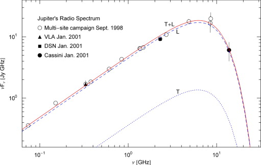
Fig. 1.

Tachyonic Cherenkov fit to the Jovian radio emission. Data points of the 1998 multi-site campaign from [2], VLA (Very Large Array), DSN (Deep Space Network) and Cassini 2001 data from [1]. The fit T + L (solid curve) depicts the total tachyonic flux density $ν F_{ν}^{T + L}$ rescaled with frequency. This unpolarized density is obtained by adding the transversal flux component $ν F_{ν}^{T}$ (dotted curve labeled T) and the longitudinal component $ν F_{ν}^{L}$ (dashed curve L), generated by a thermal electron plasma, cf. (6.2). Jupiterʼs radio spectrum shows an extended power-law ascent terminating in a spectral peak around 6 GHz, which is followed by an exponentially decaying tail inferred from the Cassini data point at 13.8 GHz. The fitting parameters are recorded in Section 6.2.

Figure options

Summarizing the flux densities employed in the spectral fit in Fig. 1, we assemble $ν^{k} F_{ν}^{T, L}$ in the above stated units. The transversal Cherenkov density (6.1) reads

equation6.2

ν^{k} F_{ν}^{T} [Jy {(GHz)}^{k}] = \frac{1.6022 \times 10^{11}}{4 π d^{2} [cm]} ν^{k} θ ({\hat{ω}}_{T, \max} (\infty) - \hat{ω}) B^{T} (ω, γ_{T, \min} (ω)),

Turn MathJax on

where

{\hat{ω}}_{T, \max} (\infty) = {(1 / (ε μ) - 1)}^{- 1 / 2}

, cf. after (5.8). The spectral function B^T

B^{T}

in (5.9) and the argument γ_T,min(ω)

γ_{T, \min} (ω)

in (5.6) are already expressed in the rescaled variable

\hat{ω} = \sqrt{ε μ_{0}} ω / m_{t}

. The longitudinal counterpart to (6.2) is obtained by replacing T→L

T \to L

and εμ→ε₀μ₀

ε μ \to ε_{0} μ_{0}

, so that

{\hat{ω}}_{L, \max} (\infty) = {(1 / (ε_{0} μ_{0}) - 1)}^{- 1 / 2}

In (6.2), we substitute $\hat{ω} = κ_{t} ν$ , where the frequency ν is measured in GHz so that κ_t=10⁹κ_t,Hz $κ_{t} = 10^{9} κ_{t, Hz}$ or, cf. after (6.1),

equation6.3

κ_{t} [s] = 10^{9} \frac{\sqrt{ε μ_{0}} h [eV s]}{m_{t} c^{2} [eV]} \approx 4.136 \times 10^{- 6} \frac{\sqrt{ε μ_{0}}}{m_{t} c^{2} [eV]} .

Turn MathJax on

In this parametrization, we find the transversal spectral function (5.9) as

equation6.4

B^{T} (ω, γ_{T, \min}) = A_{α, β} m_{t} c^{2} [eV] \frac{α_{t}}{ε \sqrt{ε μ_{0}}} \frac{ε μ}{Ω^{2} (ν)} \frac{κ_{t} ν}{κ_{t}^{2} ν^{2} + 1} \frac{1}{β^{2} γ_{T, \min}^{α + 1}} {[α (α + 1) (1 - (\frac{1}{ε μ} - 1) κ_{t}^{2} ν^{2}) - β^{2} (κ_{t}^{2} ν^{2} + 1)] {(β γ_{T, \min})}^{α + 1} Γ (- 1 - α, β γ_{T, \min}) + (1 - (\frac{1}{ε μ} - 1) κ_{t}^{2} ν^{2}) e^{- β γ_{T, \min}} (β γ_{T, \min} - α)},

Turn MathJax on

and the longitudinal spectral function in (5.10) reads

equation6.5

B^{L} (ω, γ_{L, \min}) = A_{α, β} m_{t} c^{2} [eV] \frac{α_{t}}{ε \sqrt{ε μ_{0}}} \frac{1}{Ω^{2} (ν)} \frac{κ_{t} ν}{κ_{t}^{2} ν^{2} + 1} \frac{1}{β^{2} γ_{L, \min}^{α + 1}} [α (α + 1) {(β γ_{L, \min})}^{α + 1} Γ (- α - 1, β γ_{L, \min}) + e^{- β γ_{L, \min}} (β γ_{L, \min} - α)] .

Turn MathJax on

In (6.4) and (6.5), we have to insert the frequency-dependent minimal Lorentz factors, cf. (5.6),

equation6.6

γ_{T, \min} (ν) = \frac{\sqrt{1 + κ_{t}^{2} ν^{2}}}{\sqrt{1 + κ_{t}^{2} ν^{2} (1 - 1 / (ε μ))}}, γ_{L, \min} (ν) = \frac{\sqrt{1 + κ_{t}^{2} ν^{2}}}{\sqrt{1 + κ_{t}^{2} ν^{2} (1 - 1 / (ε_{0} μ_{0}))}},

Turn MathJax on

and the scale factor

equation6.7

Ω^{2} (ν) = {(\frac{κ_{t}^{2} ν^{2}}{κ_{t}^{2} ν^{2} + 1})}^{σ}

Turn MathJax on

of the tachyonic fine-structure constant α_q(ω)=α_t/Ω²

α_{q} (ω) = α_{t} / Ω^{2}

, α_t=q²/(4πℏc)

α_{t} = q^{2} / (4 π ℏ c)

, see (5.2) and before (6.1).

The Heaviside function in the flux density (6.2) can be replaced by $θ ({\hat{ω}}_{L, T, \max} (\infty) - κ_{t} ν)$ . The highest frequency transversally/longitudinally radiated is ν_T,max=(1/(εμ)−1)^−1/2/κ_t $ν_{T, \max} = {(1 / (ε μ) - 1)}^{- 1 / 2} / κ_{t}$ and ν_L,max=(1/(ε₀μ₀)−1)^−1/2/κ_t $ν_{L, \max} = {(1 / (ε_{0} μ_{0}) - 1)}^{- 1 / 2} / κ_{t}$ respectively, cf. after (6.2). The tachyonic mass parameter κ_t $κ_{t}$ is defined in (6.3). The constant amplitudes in (6.2) and (6.4) can be combined to one fitting parameter,

equation6.8

a_{t} = \frac{1.6022 \times 10^{11}}{4 π d^{2} [cm]} m_{t} c^{2} [eV] A_{α, β} \frac{α_{t}}{ε \sqrt{ε μ_{0}}},

Turn MathJax on

with 4πd²≈4.58×10²⁸ cm²

4 π d^{2} \approx 4.58 \times 10^{28} {cm}^{2}

for Jupiter, cf. after (6.1). This amplitude a_t

a_{t}

can also be used for the longitudinal radiation component in (6.2) and (6.5).

6.2. Spectral asymptotics and tachyonic Cherenkov fit of the Jovian radio emission

We consider a thermal electron distribution (5.3) with electron index α=−2 $α = - 2$ , and permeabilities (2.1) satisfying εμ=ε₀μ₀=1 $ε μ = ε_{0} μ_{0} = 1$ . (This is slightly more general than vacuum permeabilities ε=μ=1 $ε = μ = 1$ , ε₀=μ₀=1 $ε_{0} = μ_{0} = 1$ .) The transversal spectral function B^T(ω,γ_T,min) $B^{T} (ω, γ_{T, \min})$ in (6.4) then simplifies to

equation6.9

B^{T} (ω, γ_{T, \min}) = A_{α, β} m_{t} c^{2} [eV] \frac{α_{t}}{ε \sqrt{ε μ_{0}}} \frac{1}{Ω^{2} (ν)} \frac{κ_{t} ν}{κ_{t}^{2} ν^{2} + 1} \frac{γ_{T, \min}}{β^{2}} e^{- β γ_{T, \min}} [(2 - β^{2} (κ_{t}^{2} ν^{2} + 1)) \frac{1}{β γ_{T, \min}} + 2 + β γ_{T, \min}],

Turn MathJax on

and its longitudinal counterpart in (6.5) is

equation6.10

B^{L} (ω, γ_{L, \min}) = A_{α, β} m_{t} c^{2} [eV] \frac{α_{t}}{ε \sqrt{ε μ_{0}}} \frac{1}{Ω^{2} (ν)} \frac{κ_{t} ν}{κ_{t}^{2} ν^{2} + 1} \frac{γ_{L, \min}}{β^{2}} e^{- β γ_{L, \min}} (\frac{2}{β γ_{L, \min}} + 2 + β γ_{L, \min}) .

Turn MathJax on

The minimal Lorentz factor to be substituted is

γ_{T, L, \min} (ν) = \sqrt{1 + κ_{t}^{2} ν^{2}}

, cf. (6.6), and the fine-structure scale factor Ω²(ν)

Ω^{2} (ν)

is stated in (6.7). ν is measured in GHz, and the tachyonic mass parameter κ_t

κ_{t}

is defined in (6.3).

The flux densities $ν^{k} F_{ν}^{T, L}$ in (6.2) apply, with the Heaviside function dropped. In the low-frequency limit κ_tν→0 $κ_{t} ν \to 0$ , we find the unpolarized flux

equation6.11

ν F_{ν}^{T + L} \sim A_{0} ν^{2 - 2 σ}, A_{0} = \frac{a_{t} κ_{t}^{1 - 2 σ}}{β^{3}} e^{- β} {(2 + β)}^{2} .

Turn MathJax on

The parameter a_tat $a_{t}$ is defined in (6.8). We can estimate the amplitude A₀A0 $A_{0}$ and the exponent σ by fitting this power-law slope, which is linear in a log–log plot, to the low-frequency spectrum. In the asymptotic high-frequency limit κ_tν≫1κtν≫1 $κ_{t} ν ≫ 1$ , the unpolarized flux reads

equation6.12

νFT+Lν∼A∞e−ρν(2+ρν)2,A∞=atβ3κt,ρ=βκt. $ν F_{ν}^{T + L} \sim A_{\infty} e^{- ρ ν} {(2 + ρ ν)}^{2}, A_{\infty} = \frac{a_{t}}{β^{3} κ_{t}}, ρ = β κ_{t} .$

Turn MathJax on

An initial estimate of A_∞A∞ $A_{\infty}$ and ρ is obtained by fitting this exponentially decaying flux in the high-frequency regime. Once the parameters A_0,∞A0,∞ $A_{0, \infty}$ , σ and ρ have been estimated from the asymptotic spectral fits, we find the temperature parameter β of the radiating electron population by solving

equation6.13

A0A∞ρ2σ−2=β2σ−2e−β(2+β)2. $\frac{A_{0}}{A_{\infty}} ρ^{2 σ - 2} = β^{2 σ - 2} e^{- β} {(2 + β)}^{2} .$

Turn MathJax on

This equation readily follows from the definition of the asymptotic fitting parameters A_0,∞A0,∞ $A_{0, \infty}$ and ρ in (6.11) and (6.12). Initial values for κ_tκt $κ_{t}$ and a_tat $a_{t}$ are found as κ_t=ρ/βκt=ρ/β $κ_{t} = ρ / β$ and a_t=A_∞β²ρat=A∞β2ρ $a_{t} = A_{\infty} β^{2} ρ$ .

The least-squares fit of the flux densities (6.2) is performed by varying the parameters A_0,∞,ρA0,∞,ρ $A_{0, \infty}, ρ$ and σ in the vicinity of their initial values obtained from the asymptotic fits (6.11) and (6.12); the corresponding β is obtained by solving (6.13). In addition, we may vary the permeabilities in the vicinity of εμ=ε₀μ₀=1εμ=ε0μ0=1 $ε μ = ε_{0} μ_{0} = 1$ , subject to the constraints εμ⩽1εμ⩽1 $ε μ ⩽ 1$ and ε₀μ₀⩽1ε0μ0⩽1 $ε_{0} μ_{0} ⩽ 1$ , cf. after (4.6). The electron index can also be varied around its equilibrium value α=−2α=−2 $α = - 2$ , cf. (5.3), by employing the nonthermal spectral functions (6.4) and (6.5) instead of (6.9) and (6.10), but this is not necessary for the Jovian radio spectrum.

The tachyonic Cherenkov fit of Jupiterʼs radio emission depicted in Fig. 1 is performed with a thermal electron distribution α=−2α=−2 $α = - 2$ and permeabilities εμ=ε₀μ₀=1εμ=ε0μ0=1 $ε μ = ε_{0} μ_{0} = 1$ . The numerical values of the fitting parameters are

equation6.14

σ≈0.5,β≈23.6,κt≈0.0339,at≈1.78×1012. $σ \approx 0.5, β \approx 23.6, κ_{t} \approx 0.0339, a_{t} \approx 1.78 \times 10^{12} .$

Turn MathJax on

The fine-structure scaling exponent σ is defined in (6.7), the temperature parameter β in (5.3), the tachyonic mass parameter κ_t[s]κt[s] $κ_{t} [s]$ in (6.3), and the flux amplitude a_t[eV/cm²]at[eV/cm2] $a_{t} [eV / {cm}^{2}]$ in (6.8). In practice, we use the parameters of the asymptotic flux limits (6.11) and (6.12) as fitting parameters, which are A₀≈4.9A0≈4.9 $A_{0} \approx 4.9$ , A_∞≈4.0×10⁹A∞≈4.0×109 $A_{\infty} \approx 4.0 \times 10^{9}$ , σ≈0.5σ≈0.5 $σ \approx 0.5$ and ρ≈0.8ρ≈0.8 $ρ \approx 0.8$ . The parameters in (6.14) have been calculated from these values as explained above.

The electron temperature is T[K]≈2.51×10⁸T[K]≈2.51×108 $T [K] \approx 2.51 \times 10^{8}$ , cf. after (5.4), which is the only point where the electron mass enters, via β=m_e/(k_BT)β=me/(kBT) $β = m_{e} / (k_{B} T)$ . (The mass of the radiating particle does not show in the classical Cherenkov densities (4.5), in contrast to the tachyon mass m_tmt $m_{t}$ .) Assuming vacuum permeabilities, ε≈μ≈1ε≈μ≈1 $ε \approx μ \approx 1$ , ε₀≈μ₀≈1ε0≈μ0≈1 $ε_{0} \approx μ_{0} \approx 1$ , we can estimate the tachyon mass in the radio band, m_tc²[eV]≈1.22×10⁻⁴mtc2[eV]≈1.22×10−4 $m_{t} c^{2} [eV] \approx 1.22 \times 10^{- 4}$ or m_tc²≈29.5 GHzmtc2≈29.5GHz $m_{t} c^{2} \approx 29.5 GHz$ , cf. (6.3) and (6.14). From the amplitude a_tat $a_{t}$ in (6.8) and the Jovian distance estimate, we find the product of the asymptotic tachyonic fine-structure constant α_tαt $α_{t}$ (defined before (6.1)) and the normalization factor of the electron distribution (5.3) as A_α,βα_t≈4.17×10³³Aα,βαt≈4.17×1033 $A_{α, β} α_{t} \approx 4.17 \times 10^{33}$ . The integral K_α,βKα,β $K_{α, β}$ in (5.4) determining the electron number N_e=A_α,βK_α,βNe=Aα,βKα,β $N_{e} = A_{α, β} K_{α, β}$ is calculated with the temperature parameter β in (6.14), K_α=−2,β≈6.65×10⁻¹³Kα=−2,β≈6.65×10−13 $K_{α = - 2, β} \approx 6.65 \times 10^{- 13}$ . The estimate for the product of electron count and tachyonic fine-structure constant is thus N_eα_t≈2.77×10²¹Neαt≈2.77×1021 $N_{e} α_{t} \approx 2.77 \times 10^{21}$ .

7. Conclusion

We have investigated the emission of tachyonic radiation modes by freely propagating electrons in a dispersive spacetime. The superluminal group velocity υ_T,L=dω/dk_T,L(ω) $υ_{T, L} = d ω / d k_{T, L} (ω)$ is caused by the negative mass-square in the wave numbers (3.2) of the tachyonic radiation field. υ_T,L $υ_{T, L}$ differs for transversal and longitudinal modes [14], unless the wave numbers coincide, which requires permeabilities satisfying ε₀μ₀=εμ $ε_{0} μ_{0} = ε μ$ . The tachyonic wavelength is λ_T,L=2π/k_T,L $λ_{T, L} = 2 π / k_{T, L}$ . In the radio band and with vacuum permeabilities, we find the group velocity $υ_{T, L} / c = \sqrt{ν^{2} + m_{t}^{2}} / ν$ and wavelength $λ_{T, L} [cm] \approx 29.98 / \sqrt{ν^{2} + m_{t}^{2}}$ , with ν in GHz. A tachyon mass m_t $m_{t}$ of 29.5 GHz $29.5 GHz$ is inferred from the spectral fit in Fig. 1, cf. after (6.14).

We introduced tachyonic field strengths and inductions defined by constitutive relations with frequency-dependent permeabilities. We then developed an equivalent 4D space–frequency representation of the dispersive radiation field, deriving manifestly covariant field equations. Thus the suggestive and efficient formalism of manifest covariance can be maintained, but the underlying space conception is non-relativistic, as superluminal wave propagation requires an absolute spacetime conception to preserve causality [8], [9] and [10].

We focused on superluminal Cherenkov radiation, the tachyonic radiation field being generated by a classical subluminal charge uniformly moving in a permeable spacetime. The electron mass does not enter in the classical radiation densities (4.4), which suggests that the tachyonic quanta are actually emitted by the medium stimulated by the field of the moving electron [3] and [22]. A longitudinal radiation component emerges, with amplitude proportional to the negative mass-square of the tachyonic modes. We parametrized the Cherenkov flux densities with the Lorentz factor of the inertial charge, averaged them with a relativistic electron distribution, and explained how to perform tachyonic spectral fits in the radio band.

A flux average over a mildly relativistic thermal electron population (with Maxwell–Boltzmann distribution) suffices to model the currently observed Jovian radio spectrum. We also calculated the tachyonic Cherenkov flux radiated by nonthermal electron populations (with power-law distribution), cf. Section 5, which can be useful to model X- and γ-ray spectra [23], [24] and [25]. As for Jupiter, the low flux density at 13.8 GHz (Cassini 2001 in-situ measurement [1] and [26]) is caused by an exponential spectral cutoff. The low-frequency spectrum is linear in the double-logarithmic flux representation of Fig. 1. The cross-over region around the spectral peak at 6 GHz is also well reproduced by the tachyonic flux densities (4.4) averaged over a thermal electron population.

References

- [1]
- S.J. Bolton et al.
- Nature, 415 (2002), p. 987
- View Record in Scopus
  |
  Full Text via CrossRef
  | Cited By in Scopus (44)
- [2]
- I. de Pater et al.
- Icarus, 163 (2003), p. 434
- Article
  |
  PDF (466 K)
  |
  View Record in Scopus
  | Cited By in Scopus (19)
- [3]
- L.D. Landau, E.M. Lifshitz
- Electrodynamics of Continuous Media
- Pergamon, Oxford (1984)
- [4]
- V.L. Ginzburg, V.N. Tsytovich
- Transition Radiation and Transition Scattering
- Hilger, Bristol (1990)
- [5]
- B.M. Bolotovskiĭ, V.L. Ginzburg
- Sov. Phys. Usp., 15 (1972), p. 184
- [6]
- G.N. Afanasiev, M.V. Lyubchenko, Yu.P. Stepanovsky
- Proc. R. Soc. A, Math. Phys. Eng. Sci., 462 (2006), p. 689
- View Record in Scopus
  | Cited By in Scopus (3)
- [7]
- R. Tomaschitz
- Phys. Lett. A, 377 (2013), p. 945
- Article
  |
  PDF (247 K)
  |
  View Record in Scopus
  | Cited By in Scopus (1)
- [8]
- R. Tomaschitz
- Europhys. Lett., 97 (2012), p. 39003
- View Record in Scopus
  |
  Full Text via CrossRef
  | Cited By in Scopus (1)
- [9]
- R. Tomaschitz
- Europhys. Lett., 98 (2012), p. 19001
- View Record in Scopus
  |
  Full Text via CrossRef
  | Cited By in Scopus (1)
- [10]
- R. Tomaschitz
- Europhys. Lett., 102 (2013), p. 61002
- Full Text via CrossRef
- [11]
- R. Tomaschitz
- Eur. Phys. J. C, 69 (2010), p. 241
- View Record in Scopus
  |
  Full Text via CrossRef
  | Cited By in Scopus (5)
- [12]
- R. Tomaschitz
- Physica A, 320 (2003), p. 329
- Article
  |
  PDF (315 K)
  |
  View Record in Scopus
  | Cited By in Scopus (16)
- [13]
- R. Tomaschitz
- Opt. Commun., 282 (2009), p. 1710
- Article
  |
  PDF (321 K)
  |
  View Record in Scopus
  | Cited By in Scopus (5)
- [14]
- R. Tomaschitz
- Physica B, 404 (2009), p. 1383
- Article
  |
  PDF (291 K)
  |
  View Record in Scopus
  | Cited By in Scopus (7)
- [15]
- R. Tomaschitz
- Appl. Phys. B, 101 (2010), p. 143
- View Record in Scopus
  |
  Full Text via CrossRef
- [16]
- R. Tomaschitz
- Physica A, 385 (2007), p. 558
- Article
  |
  PDF (276 K)
  |
  View Record in Scopus
  | Cited By in Scopus (10)
- [17]
- R. Tomaschitz
- Physica A, 387 (2008), p. 3480
- Article
  |
  PDF (693 K)
  |
  View Record in Scopus
  | Cited By in Scopus (9)
- [18]
- R. Tomaschitz
- Physica B, 405 (2010), p. 1022
- Article
  |
  PDF (370 K)
  |
  View Record in Scopus
  | Cited By in Scopus (5)
- [19]
- R. Tomaschitz
- Physica A (2013) http://dx.doi.org/10.1016/j.physa.2013.09.068
- [20]
- R. Tomaschitz
- Ann. Phys., 322 (2007), p. 677
- Article
  |
  PDF (347 K)
  |
  View Record in Scopus
  | Cited By in Scopus (15)

- [21]
- K. Nakamura et al.
- J. Phys. G, 37 (2010), p. 075021
- View Record in Scopus
  |
  Full Text via CrossRef
  | Cited By in Scopus (227)
- [22]
- R. Tomaschitz
- Class. Quantum Grav., 18 (2001), p. 4395
- View Record in Scopus
  |
  Full Text via CrossRef
  | Cited By in Scopus (20)
- [23]
- A. Bhardwaj et al.
- J. Geophys. Res., 111 (2006), p. A11225
- View Record in Scopus
  |
  Full Text via CrossRef
  | Cited By in Scopus (4)
- [24]
- G. Branduardi-Raymont et al.
- Astron. Astrophys., 463 (2007), p. 761
- View Record in Scopus
  |
  Full Text via CrossRef
  | Cited By in Scopus (30)
- [25]
- G. Branduardi-Raymont et al.
- Planet. Space Sci., 55 (2007), p. 1126
- Article
  |
  PDF (1333 K)
  |
  View Record in Scopus
  | Cited By in Scopus (13)
- [26]
- J.L. Kloosterman et al.
- Icarus, 193 (2008), p. 644
- Article
  |
  PDF (434 K)
  |
  View Record in Scopus
  | Cited By in Scopus (1)

Tachyonic Cherenkov emission from Jupiterʼs radio electrons

Highlights

Abstract

Keywords

1. Introduction

2. Tachyonic Proca–Maxwell fields: manifestly covariant field equations in a permeable spacetime

3. Asymptotic radiation fields: time-averaged transversal and longitudinal energy flux

4. Superluminal radiation by an inertial charge in a dispersive spacetime

5. Tachyonic Cherenkov densities averaged with relativistic electron distributions

6. Tachyonic spectral fit to Jupiterʼs radio emission

6.1. Superluminal Cherenkov flux in the radio band

6.2. Spectral asymptotics and tachyonic Cherenkov fit of the Jovian radio emission

7. Conclusion

References

Bibliographic information

Article history

Applications and tools

Workspace