![Flux density of cosmic-ray electrons. Data points from AMS-02 [1] (open ...](FT_stationary_non-equilibrium_plasma_of_cosmic-ray_electrons_and_positrons_files/1-s2_102.gif "Flux density of cosmic-ray electrons. Data points from AMS-02 [1] (open ...")


The stationary non-equilibrium plasma of cosmic-ray electrons and positrons


Highlights
- •
The thermodynamic variables of the cosmic-ray electron–positron plasma are calculated.
- •
Spectral fits to the AMS-02 and HESS GeV–TeV electron and positron fluxes are performed.
- •
A semi-empirical phase-space reconstruction of the partial probability densities is carried out.
- •
Partition function & entropy of a relativistic plasma in stationary non-equilibrium are derived.
- •
The positron fraction extrapolated to TeV energies shows a broad peak & exponential decay.
Abstract
The statistical properties of the two-component plasma of cosmic-ray electrons and positrons measured by the AMS-02 experiment on the International Space Station and the HESS array of imaging atmospheric Cherenkov telescopes are analyzed. Stationary non-equilibrium distributions defining the relativistic electron–positron plasma are derived semi-empirically by performing spectral fits to the flux data and reconstructing the spectral number densities of the electronic and positronic components in phase space. These distributions are relativistic power-law densities with exponential cutoff, admitting an extensive entropy variable and converging to the Maxwell–Boltzmann or Fermi–Dirac distributions in the non-relativistic limit. Cosmic-ray electrons and positrons constitute a classical (low-density high-temperature) plasma due to the low fugacity in the quantized partition function. The positron fraction is assembled from the flux densities inferred from least-squares fits to the electron and positron spectra and is subjected to test by comparing with the AMS-02 flux ratio measured in the GeV interval. The calculated positron fraction extends to TeV energies, predicting a broad spectral peak at about 1 TeV followed by exponential decay.
Keywords
- Stationary non-equilibrium distributions;
- Cosmic-ray electron–positron plasma;
- Relativistic statistical ensembles;
- Power-law densities with exponential cutoff;
- Nonthermal ensemble averaging;
- Classical & quantum partitions with extensive entropy
1. Introduction
We study the statistical mechanics of the cosmic-ray electron–positron plasma, based on high-precision spectra obtained with the Alpha Magnetic Spectrometer (AMS-02) [1] and [2]. We demonstrate that this plasma can be treated, in close analogy to the photon gas of the cosmic microwave background radiation, as a primordial electron gas in stationary non-equilibrium. A primordial origin is also suggested by the high isotropy of the observed fluxes. Primordiality of the cosmic-ray electron–positron plasma is tantamount to the material realization of a universal cosmic reference frame as the rest frame of a relativistic gas of massive particles. An alternative approach is to use relativistic kinetic theory, but to arrive at quantitative densities suitable for spectral fitting, one has to specify production mechanisms and interaction processes with cosmic matter and radiation fields which are uncertain [3].
We perform spectral fits to the AMS-02 electron and positron fluxes and reconstruct, from the inferred spectral densities, the distribution functions of the electronic and positronic plasma components. The partial number densities are relativistic non-equilibrium distributions, exponentially cut power-law densities [4] and [5] which converge to the Maxwell–Boltzmann distribution for low particle velocities, the Coulomb interaction being negligible. We calculate the classical partition function, by ensemble averaging in phase space, and the entropy function which is an extensive variable. We then quantize the grand partition function and show, based on the fugacity obtained from the spectral fits, that the classical limit is realized. Finally we calculate the positron fraction and give estimates of the thermodynamic parameters of this low-density high-temperature plasma.
In Section 2, we consider a relativistic plasma in stationary non-equilibrium and relate the classical spectral number density to the empirical flux density obtained from spectral fits to the measured electron and positron fluxes (performed in Section 5). In Section 3, we derive the thermodynamic variables of the electronic and positronic plasma components in phase space, based on probability distributions inferred from the spectral fits, in particular the electronic/positronic energy and entropy densities.
In Section 4, we explain the quantization of the classical nonthermal partition function and demonstrate that the classical limit applies to the cosmic-ray electron–positron plasma due to the small fugacity. The formalism developed in Sections 2, 3 and 4 is based on relativistic dispersion relations and designed to be practically suitable for spectral fits in any energy range. Foundational aspects of relativistic statistical mechanics and thermodynamics such as the arrow of time and entropy are discussed in Refs. [6], [7], [8] and [9]. Recent applications of relativistic statistical mechanics include the quark–gluon plasma [10] and [11], plasmas in gravitational fields [12], gases of neutral particles with long-range spin–spin interaction [13] and condensation effects in relativistic Bose–Einstein gases [14]. Kinetic theory with relativistic dispersion relations, in particular the relativistic Boltzmann equation in Grad’s moment expansion and Chapman–Enskog approximation, is discussed in Refs. [15] and [16] and a relativistic version of the Fokker–Planck equation in Ref. [17].
In Section 5, we perform least-squares fits to the AMS-02 and HESS [18] electron and positron spectra. The measured spectra are located in the GeV and low TeV range, where we can use the ultra-relativistic approximation of the spectral densities derived in Sections 2, 3 and 4, which means to drop the mass term in the electronic dispersion relation. The ultra-relativistic electronic/positronic flux densities obtained in this way are then used to assemble the positron fraction, which has been measured by the AMS-02 Collaboration in the GeV range [19], thus providing a test of the spectral number densities on which the thermodynamic variables are based. Extrapolation of the analytic formula for the positron fraction into the TeV range suggests an extended spectral peak centered around 1 TeV and exponential decay above 10 TeV.
As mentioned, this primordial approach to the cosmic-ray electron–positron plasma is alternative to the use of kinetic equations which require the assumption of specific electron/positron production mechanisms [20]. A possible mechanism is electron/positron emission caused by interaction of high-energy protons or heavier cosmic-ray nuclei with the interstellar medium [3] and [21]. Quantitative models thereof turn out to be inconsistent with the pronounced rise of the positron fraction, so that additional positron sources have to be invoked, for instance, discrete high-energy sources such as pulsar magnetospheres or the shocked plasmas of supernova remnants [22], even if isotropy is somewhat compromised. Other authors prefer positron production via decay or annihilation of a variety of hypothetical dark matter particles at TeV energies [23] which could exist in galactic halos.
In Section 5, we also give estimates of the specific energy and number densities, entropy production, temperature, fugacity and chemical potential of the electronic/positronic plasma components. We calculate the specific densities of the actually measured electrons/positrons in the energy range above 1 GeV up to low TeV energies where an exponential cutoff occurs. We then restore the electron mass in the dispersion relation and extrapolate the analytic spectral densities obtained from the spectral fits to lower energies. In this way, we can predict the specific energy, number and entropy densities of the complete statistical ensemble comprising all gas particles by integrating the electronic/positronic spectral densities down to the electron mass. In Section 6, we present our conclusions.
2. Relativistic plasma in stationary non-equilibrium
We start with the classical number density of a free electron plasma,
The number density (2.1) is assembled with the integration measure ![]() and the dispersion relation for free relativistic particles
and the dispersion relation for free relativistic particles ![]() , so that
, so that ![]() . The normalization factor s/(2π)3 arises from box quantization in the continuum limit, see (4.4). The quantized spectral density of which (2.1) is the classical limit is discussed in Section 4. Density (2.1) is thus assembled as
. The normalization factor s/(2π)3 arises from box quantization in the continuum limit, see (4.4). The quantized spectral density of which (2.1) is the classical limit is discussed in Section 4. Density (2.1) is thus assembled as ![]() , with the normalized spectral function G(E)=g(E)/g(m). The non-relativistic limit of
, with the normalized spectral function G(E)=g(E)/g(m). The non-relativistic limit of ![]() is thermal since
is thermal since ![]() , where υ≪1
is the particle speed parametrizing the non-relativistic
Maxwell–Boltzmann distribution, whose chemical potential is obtained
from the relativistic potential
, where υ≪1
is the particle speed parametrizing the non-relativistic
Maxwell–Boltzmann distribution, whose chemical potential is obtained
from the relativistic potential ![]() by subtraction of the rest mass m.
by subtraction of the rest mass m.
The spectral flux density is found by multiplying the number density with the group velocity, ![]() . The flux density per steradian is thus
. The flux density per steradian is thus
In flux density (2.4), we specified the spectral function g(E) in (2.3) by the ansatz
The number of particles in a volume V with energies exceeding ![]() is calculated as
is calculated as
Entropy is an extensive quantity proportional to V,
To demonstrate thermodynamic stability, we first show that the inequalities 0≤CV≤CP hold for the isochoric and isobaric heat capacities. To this end, we note, cf. (2.7) and (2.8),
We also have to show mechanical stability, 0≤κS≤κT, where κS and κT denote adiabatic and isothermal compressibility. Since ![]() , cf. (2.7), the thermal equation of state reads P=N/(βV), and the isothermal compressibility is thus κT=−(1/V)∂V(β,P,N)/∂P=1/P. The adiabatic compressibility is related to the heat capacities by κS=κTCV/CP, which implies the stated inequalities since κT>0 and CP>CV. This holds true for the electronic and positronic plasma components alike.
, cf. (2.7), the thermal equation of state reads P=N/(βV), and the isothermal compressibility is thus κT=−(1/V)∂V(β,P,N)/∂P=1/P. The adiabatic compressibility is related to the heat capacities by κS=κTCV/CP, which implies the stated inequalities since κT>0 and CP>CV. This holds true for the electronic and positronic plasma components alike.
3. Thermodynamic variables in phase space
We consider the phase space of n electrons with measure

The phase-space probability is normalized to one,


4. Quantized partition function of the electronic and positronic plasma components
The quantized version of the classical partition function ![]() in (2.7) is obtained by a trace calculation in fermionic occupation number representation [25] and [27],
in (2.7) is obtained by a trace calculation in fermionic occupation number representation [25] and [27],
With these prerequisites, trace (4.1) can be evaluated as

5. Spectral fits to high-energy cosmic-ray electron and positron fluxes
The spectral fits in Fig. 1 and Fig. 2 are performed in the GeV and TeV range, the ultra-relativistic regime, so that we can drop the factor (1−m2/E2) in the flux density, see the discussion following Eq. (2.4),
![Flux density of cosmic-ray electrons. Data points from AMS-02 [1] (open ...](FT_stationary_non-equilibrium_plasma_of_cosmic-ray_electrons_and_positrons_files/1-s2_002.jpg)
- Fig. 1.
Flux density of cosmic-ray electrons. Data points from AMS-02 [1] (open circles) and HESS [18] (open squares). The HESS points refer to the combined electron and positron flux and are rescaled by a factor of 0.6 to obtain a continuous transition to the AMS-02 electron flux. The solid curve is a fit of the ultra-relativistic electronic flux density
 in (5.1), the fitting parameters are listed in Table 1. The error band defined by the dotted curves indicates the 2σ (95%) confidence limits of the least-squares fit,
  .
The residuals are depicted in the lower panel. The thermodynamic
parameters of the electronic and positronic plasma components are
recorded in Table 2.
.
The residuals are depicted in the lower panel. The thermodynamic
parameters of the electronic and positronic plasma components are
recorded in Table 2.
- Table 1.
Fitting parameters of the electronic (
 ) and positronic (
 ) flux densities. The spectral fits depicted in Fig. 1 and Fig. 2 are performed with the ultra-relativistic flux density
  , cf. (2.4) and (5.1). Listed are the flux amplitude AΦ, the power-law exponents α1,β1,γ1, the power-law amplitudes b1,c1, and the temperature parameter β in the exponential. Derived thermodynamic parameters of the electronic/positronic plasma components are recorded in Table 2.
α1 b1 (GeV) β1 c1 (GeV) γ1 
21.34 ± 0.617 2.134 ± 0.050 3.584 ± 0.119 2.453 ± 0.035 329.1 ± 62.80 1.074 ± 0.131 1.127 ± 0.137 1.966 ± 0.102 2.081 ± 0.144 2.524 ± 0.227 2.272 ± 0.080 51.30 ± 30.35 0.881 ± 0.044 1.200 ± 0.107 - Full-size table
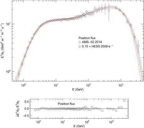
- Fig. 2.
Spectral flux density of the positronic plasma component. Data points from AMS-02 [1] (open circles) and HESS [18] (open squares). The caption to Fig. 1 applies. HESS flux points are rescaled by a factor of 0.15. The χ2 fit (solid curve,
 ) is based on the spectral flux density
  in (5.1); the fitting parameters are listed in Table 1. The dotted curves depict the 2σ
confidence limits, the residuals are shown in the lower panel. The
highest energy HESS data point lies outside the error band, suggesting
the possibility of a subexponential Weibull-type spectral decay [37], [38], [39] and [40],
but this hinges on one flux point with large error bar. Preliminary
estimates of the combined electron–positron flux in the low TeV region
obtained with the PAMELA calorimeter [41] also indicate an exponential cutoff as depicted in Fig. 1 and Fig. 2.
in (5.1); the fitting parameters are listed in Table 1. The dotted curves depict the 2σ
confidence limits, the residuals are shown in the lower panel. The
highest energy HESS data point lies outside the error band, suggesting
the possibility of a subexponential Weibull-type spectral decay [37], [38], [39] and [40],
but this hinges on one flux point with large error bar. Preliminary
estimates of the combined electron–positron flux in the low TeV region
obtained with the PAMELA calorimeter [41] also indicate an exponential cutoff as depicted in Fig. 1 and Fig. 2.
- Table 2.
Thermodynamic parameters of the cosmic-ray electron–positron plasma, cf. (5.2) and Table 1.
 is the specific number density and
  the specific energy density of the electronic/positronic component, cf. (5.3). Also recorded are temperature T, fugacity z, chemical potential μ and the specific entropy density
  ; the entropy production mainly stems from the fugacity term
  in (5.4) (α=−logz). The specific densities
  and are listed for two lower threshold energies
  of the electron/positron spectrum. The cutoff energy of 1 GeV (1st
and 3rd row) refers to specific densities comprising GeV and low-TeV
electrons/positrons as measured by the AMS-02 spectrometer and the HESS
Cherenkov array. The spectral densities (5.2) obtained from the fits in Fig. 1 and Fig. 2 can be extrapolated to lower energies; in the 2nd and 4th row, we identify with the electron mass and list the total specific densities, cf. after (5.4).
of the electron/positron spectrum. The cutoff energy of 1 GeV (1st
and 3rd row) refers to specific densities comprising GeV and low-TeV
electrons/positrons as measured by the AMS-02 spectrometer and the HESS
Cherenkov array. The spectral densities (5.2) obtained from the fits in Fig. 1 and Fig. 2 can be extrapolated to lower energies; in the 2nd and 4th row, we identify with the electron mass and list the total specific densities, cf. after (5.4). - (GeV)


 (GeV)
(GeV)logz μ (GeV) 
1 1.30×10⁻⁶ 4.17×10⁻⁶ 888 −98.4 −8.73×10 4 1.30×10⁻⁴ 0.511×10⁻³ 5.43×10⁻⁶ 4.95×10⁻⁶ 888 −98.4 −8.73×10 4 5.40×10⁻⁴ 1 9.15×10⁻⁸ 2.75×10⁻⁷ 833 −100 −8.36×10 4 9.28×10⁻⁶ 0.511×10⁻³ 5.43×10⁻⁷ 3.50×10⁻⁷ 833 −100 −8.36×10 4 5.51×10⁻⁵ - Full-size table
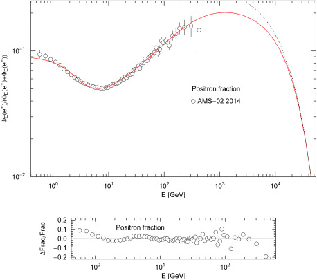
- Fig. 3.
Positron fraction of the cosmic-ray electron–positron plasma. Depicted is the flux ratio
 (solid curve). The electronic/positronic flux densities
  and
and  are stated in (5.1) with parameters in Table 1 (obtained from the χ2 fits in Fig. 1 and Fig. 2). The data points (open circles) show the AMS-02 positron fraction [19]. The dotted curve is the exponentially decaying asymptotic limit of the positron fraction, see after (5.1). The residuals are plotted in the lower panel.
The classical spectral number density reads, cf. (2.1) and Refs. [33] and [34],
6. Conclusion
We developed a statistical description of the cosmic-ray electron–positron plasma based on stationary non-equilibrium distributions. The latter are inferred from spectral fits to the electron and positron spectra measured by the AMS-02 experiment in the GeV interval and the Cherenkov telescope HESS in the low TeV range. In particular, we do not need to make hypothetical assumptions on sources and production mechanisms of high-energy cosmic-ray electrons/positrons. Their spectral number densities are semi-empirically reconstructed from the measured electron and positron fluxes as classical ensemble averages in phase space.
The
cosmic-ray electron–positron plasma is relativistic and nonthermal, the
Coulomb interaction can be neglected due to the low particle density
and high temperature. The criterion for this approximation is a small
ratio ![]() , where
, where ![]() is the interparticle distance and e2/(4π)≈1/137 the fine-structure constant [35] and [36]. In the case of cosmic-ray electrons and positrons, this ratio is of order 10−23. Temperature and the specific number density
is the interparticle distance and e2/(4π)≈1/137 the fine-structure constant [35] and [36]. In the case of cosmic-ray electrons and positrons, this ratio is of order 10−23. Temperature and the specific number density ![]() of the non-equilibrated plasma components are listed in Table 2. Quantum corrections to the classical partition function are also negligible, cf. after (4.7).
of the non-equilibrated plasma components are listed in Table 2. Quantum corrections to the classical partition function are also negligible, cf. after (4.7).
The entropy of the cosmic-ray electron–positron plasma is an extensive quantity, even though the underlying electronic/positronic probability distributions are nonthermal. We also checked the positivity of the heat capacities and compressibility, which ensures the thermodynamic stability of each plasma component implying positive root mean squares of the thermodynamic variables. The thermal Maxwell–Boltzmann distribution is recovered in the non-relativistic limit of the spectral number density (2.1).
To summarize the approximations, cosmic-ray electrons and positrons at GeV energies and beyond constitute a relativistic gas, so that one has to use relativistic dispersion relations. As the particles are charged, they constitute a two-component plasma, but since the gas is dilute and thus the interparticle distances large according to the number densities in Table 2, one can ignore Coulomb interaction and Debye screening, see the estimate above. As the fugacity is low, the quantum distribution (4.7) can be approximated by its classical limit. In the spectral fits in Section 5, the ultra-relativistic approximation is used, because the electronic mass/energy ratio is negligible in the GeV band, cf. after (2.4). In the calculation of the specific thermodynamic densities of the electronic and positronic gas components, cf. Table 2, we restored this ratio in the electronic dispersion relation, since the fitted spectral densities determining the specific densities are extrapolated to lower energies, see the remarks after (5.4).
We calculated the positron fraction using the parameters obtained from the spectral fits in Fig. 1 and Fig. 2, and compared it with the AMS-02 fraction measured in the GeV range. As the analytic representation (5.1) of the electronic/positronic flux densities also applies at TeV energies and since the temperature of the positronic plasma component is lower than of the electrons, cf. Table 1, we predict a broad spectral peak of the positron fraction at around 1 TeV which is followed by exponential decay, see after (5.1) and Fig. 3.
References
- [1]
Phys. Rev. Lett., 113 (2014), Article 121102

- [2]
J. Phys.: Conf. Ser., 631 (2015), Article 012046
- [3]
Astropart. Phys., 39 (2012), p. 2
- [4]
Physica A, 427 (2015), p. 1
- [5]
Physica A, 412 (2014), p. 32
- [6]
Physica A, 106 (1981), p. 204
- [7]
Physica A, 194 (1993), p. 1
- [8]
Physica A, 88 (1977), p. 425
- [9]
Physica A, 307 (2002), p. 375
- [10]
Physica A, 392 (2013), p. 4388
- [11]
Physica A, 432 (2015), p. 71
- [12]
Physica A, 393 (2014), p. 76
- [13]
Physica A, 432 (2015), p. 108
- [14]
Physica A, 391 (2012), p. 5422
- [15]
Physica A, 381 (2007), p. 8
- [16]
Physica A, 389 (2010), p. 4580
- [17]
Physica A, 439 (2015), p. 34
- [18]
Phys. Rev. Lett., 101 (2008), Article 261104
- [19]
Phys. Rev. Lett., 113 (2014), Article 121101
- [20]
J. Phys.: Conf. Ser., 632 (2015), Article 012027
- [21]
EPJ Web Conf., 99 (2015), p. 14001
- [22]
Phys. Lett. B, 749 (2015), p. 267
- [23]
Phys. Lett. B, 747 (2015), p. 495
- [24]
Physica A, 385 (2007), p. 558
- [25]
Physica A, 387 (2008), p. 3480
- [26]
Phys. Rep., 149 (1987), p. 91
- [27]
Physica B, 405 (2010), p. 1022
- [28]
Phys. Rev. Lett., 106 (2011), Article 201101
- [29]
Phys. Rev. Lett., 111 (2013), Article 081102
- [30]
Phys. Rev. Lett., 108 (2012), Article 011103
- [31]
Phys. Rev. D, 82 (2010), Article 092004
- [32]
Astron. Astrophys., 508 (2009), p. 561
- [33]
Europhys. Lett., 104 (2013), p. 19001
- [34]
Physica A, 394 (2014), p. 110
- [35]
Rev. Modern Phys., 54 (1982), p. 1017
- [36]
Rev. Mod. Phys., 65 (1993), p. 255
- [37]
Europhys. Lett., 106 (2014), p. 39001
- [38]
Phys. Lett. A, 378 (2014), p. 2337
- [39]
Phys. Lett. A, 378 (2014), p. 2915
- [40]
J. High Energy Astrophys., 8 (2015), p. 10
- [41]
J. Phys.: Conf. Ser., 632 (2015), p. 012014