doi:10.1209/0295-5075/84/19001
Polarization of superluminal γ-rays:
Tachyonic flare spectra of quasar 3C 279
R. Tomaschitz
Department of Physics, Hiroshima University - 1-3-1 Kagami-yama, Higashi-Hiroshima 739-8526, Japan
E-mail: tom@geminga.org
Received 20 August 2008, accepted for publication 29 August
2008
Published 17 September 2008
| Abstract. The
polarization of
superluminal radiation is studied, based on the tachyonic Maxwell
equations for Proca fields with negative mass-square. The
cross-sections for the scattering of transversal and longitudinal
tachyons by electrons are derived. The polarized superluminal flux
vectors of dipole currents are calculated, and the power transversally
and longitudinally radiated is obtained. Specifically, the polarization
of the γ-ray spectrum of quasar 3C 279 is studied. Two flare spectra of
this blazar at redshift 0.538 are fitted with tachyonic cascades
generated by the thermal electron plasma in the active galactic
nucleus. The transversal and longitudinal radiation components and the
thermodynamic parameters of the ultra-relativistic plasma are extracted
from the spectral map. An extended spectral plateau typical for
tachyonic γ-ray spectra emerges in the MeV and low GeV range. The
curvature of the adjacent GeV spectral slope is shown to be intrinsic,
caused by the Boltzmann factor of the electron plasma rather than by
intergalactic absorption.
PACS numbers: 95.30.Gv, 13.88.+e, 42.25.Ja |
Introduction
We point out evidence for superluminal γ-rays in the spectral
map of the radio quasar 3C 279 at redshift z  0.538, cf.
refs. [1–4].
In contrast to GeV-TeV photons, the extragalactic tachyon flux is not
attenuated by interaction with the cosmic background light. There is no
absorption of tachyonic γ-rays via pair creation, as tachyons do not
interact with infrared background photons. We show that the curvature
in the GeV flare spectrum of this distant blazar is intrinsic, caused
by the Boltzmann factor of the thermal electron plasma generating the
radiation, and reproduced by a tachyonic cascade fit. The cascades are
obtained by averaging the superluminal spectral densities of individual
electrons with ultra-relativistic thermal electron
distributions [5,
6]. The tachyonic
radiation field is a real Proca field with negative
mass-square [7].
The negative mass-square refers to the radiation field rather than the
current, in contrast to the traditional approach assuming superluminal
source particles emitting electromagnetic radiation [8, 9],
and causes striking differences compared to electrodynamics. Apart from
the superluminal speed of the tachyonic quanta, the radiation is
partially longitudinally polarized, the gauge freedom is broken, and
freely propagating charges can radiate superluminal quanta [10–13].
0.538, cf.
refs. [1–4].
In contrast to GeV-TeV photons, the extragalactic tachyon flux is not
attenuated by interaction with the cosmic background light. There is no
absorption of tachyonic γ-rays via pair creation, as tachyons do not
interact with infrared background photons. We show that the curvature
in the GeV flare spectrum of this distant blazar is intrinsic, caused
by the Boltzmann factor of the thermal electron plasma generating the
radiation, and reproduced by a tachyonic cascade fit. The cascades are
obtained by averaging the superluminal spectral densities of individual
electrons with ultra-relativistic thermal electron
distributions [5,
6]. The tachyonic
radiation field is a real Proca field with negative
mass-square [7].
The negative mass-square refers to the radiation field rather than the
current, in contrast to the traditional approach assuming superluminal
source particles emitting electromagnetic radiation [8, 9],
and causes striking differences compared to electrodynamics. Apart from
the superluminal speed of the tachyonic quanta, the radiation is
partially longitudinally polarized, the gauge freedom is broken, and
freely propagating charges can radiate superluminal quanta [10–13].
In the second section, we discuss the tachyonic Maxwell equations for Proca fields with negative mass-square, as well as the tachyon flux generated by dipole currents, and the power transversally and longitudinally radiated. In the third section, the polarization of tachyonic dipole radiation is investigated, and the Thomson cross-sections for the scattering of polarized tachyons by electrons are derived. The polarization of the tachyonic γ-ray spectrum of the active galactic nucleus 3C 279 is studied in the fourth section. We perform a tachyonic cascade fit to two flare spectra of this blazar, and extract the thermodynamic parameters of the electron plasma as well as the transversal and longitudinal flux components from the least-squares fit. The γ-ray flares were recorded with the EGRET and COMPTEL instruments on board the Compton Gamma Ray Observatory in June 1991 [2, 3], and the ground-based imaging atmospheric Cherenkov detector MAGIC in January–April 2006 [4]. The conclusions are summarized in the fifth section.
Superluminal flux and power
Proca fields with negative mass-square and tachyonic Maxwell equations
The tachyonic radiation field in vacuum is a real vector field
with negative mass-square, satisfying the Proca equation, (∂ν∂ν + mt2)Aμ = −jμ,
subject to the Lorentz condition A,μμ = 0.
The mass term is added with a positive sign, and the sign convention
for the metric defining the d'Alembertian is diag(−1, 1, 1, 1), so that
mt2 > 0
is the negative mass-square of the radiation field. The
tachyon-electron mass ratio is mt/m 1/238, and
the ratio of tachyonic
and electric fine-structure constants reads q2/e2 1.4 × 10⁻¹¹,
both inferred from hydrogenic Lamb shifts [7]. q is
the tachyonic charge carried by the subluminal electron current jμ = (ρ,
j).
As for the spectral fit in the fourth section, the tachyon-electron
mass ratio enters in the cutoff energy of the tachyonic cascades, cf.
caption to fig. 1.
The wave equation in conjunction with the Lorentz condition is
equivalent to the tachyonic Maxwell equations

In Fourier space,  , the field equations read

where the amplitudes of the field strengths and potentials
are connected by  and
and  .
.
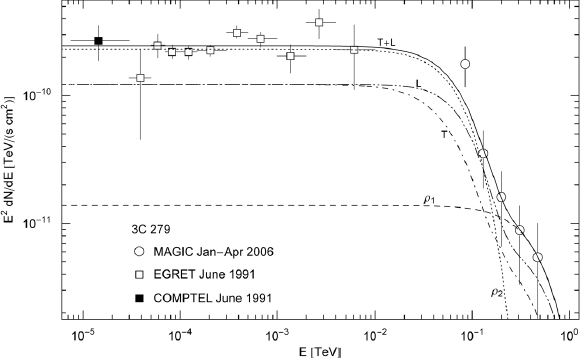
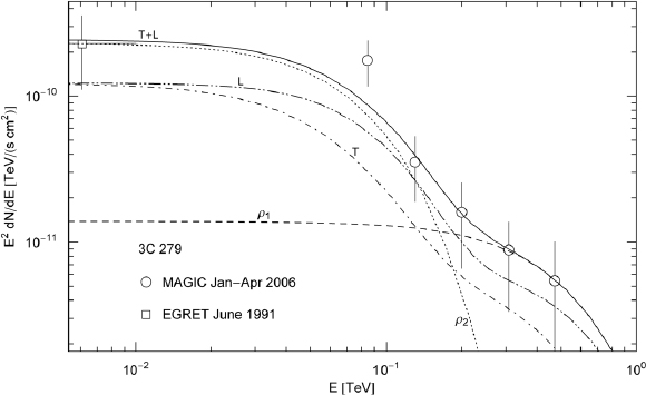
| Figure 1.
γ-ray broadband of quasar 3C 279. MAGIC flux points from ref. [4], EGRET points from
ref. [2], COMPTEL
point from ref. [3].
The solid line T + L depicts the unpolarized
differential tachyon flux dNT+L/dE,
obtained by adding the flux densities ρ1,2 of
two ultra-relativistic electron populations, cf. table 1, and rescaled with E2
for better visibility of the spectral curvature, cf. (16). The transversal (T,
dot-dashed line) and longitudinal (L, double-dot–dashed line) flux
densities dNT,L/dE
add up to the total unpolarized flux T + L. The
exponential decay of the cascades ρ1,2 sets in
at about Ecut (mt/m)kT,
implying cutoffs at 180 GeV for the ρ1
cascade and 29 GeV for ρ2. The EGRET
points define a spectral plateau in the MeV to GeV range typical for
tachyonic cascade spectra [15,
16, 21].
The least-squares fit is done with the unpolarized tachyon flux
T + L, and subsequently split into transversal and
longitudinal components. |
Tachyonic Poynting vectors of dipole currents
We consider a dipole current j(x,
t) = pδ(x)e−iω0t + c.c.,
with constant dipole vector p, and use a truncated
Fourier representation,  , as well as the truncated delta function
  , to find

In this way, a well-defined meaning is given to squares of delta functions arising in the flux vectors, owing to the T → ∞ limit 2πδ2(ω;T)/T → δ(ω).
The transversal and longitudinal current transforms  defining the asymptotic outgoing wave fields are calculated via

where  is the tachyonic wave number. The
projection of
is the tachyonic wave number. The
projection of  onto a right-handed triad of polarization vectors
  and n
of the radiation field gives the transversal and longitudinal current
components
and n
of the radiation field gives the transversal and longitudinal current
components

Here, n = x/r
is the longitudinal polarization vector, and the  define two degrees of linear transversal
polarization, so that
define two degrees of linear transversal
polarization, so that  and n
constitute an orthonormal triad. The outgoing polarized field
components are asymptotic solutions of the tachyonic Maxwell equations,
and n
constitute an orthonormal triad. The outgoing polarized field
components are asymptotic solutions of the tachyonic Maxwell equations,
 , with amplitudes generated by the dipole
current (3),
, with amplitudes generated by the dipole
current (3),

The time-averaged transversal and longitudinal Poynting vectors are assembled as [11]
The total transversal flux  ST
ST is obtained by adding
the transversal
polarization components ST(i). The polarized flux
components radiated by
a dipole current read
is obtained by adding
the transversal
polarization components ST(i). The polarized flux
components radiated by
a dipole current read

Power transversally and longitudinally radiated
The power radiated into the solid angle
dΩ = sin θ dθ d is dPT,L = nST,Lr2dΩ,
where we substitute the flux vectors (8)
to find the power differentials of the dipole current (3),
is dPT,L = nST,Lr2dΩ,
where we substitute the flux vectors (8)
to find the power differentials of the dipole current (3),

Integration over the solid angle gives the total transversal/longitudinal power components,

which also apply for a complex dipole vector, as there are no interference terms arising in the averaged flux vectors.
The dipole approximation of a monochromatic current  is obtained by replacing
  by pδ(x), with
  . Invoking current conservation,
  , we write p = −iωd,
with dipole moment
, we write p = −iωd,
with dipole moment  , and substitute
  in (10).
Regarding the dipole, we consider an oscillating tachyonic charge with
velocity
in (10).
Regarding the dipole, we consider an oscillating tachyonic charge with
velocity  , so that
  ,
cf. before (1). The
power radiated in transversal linear polarization
,
cf. before (1). The
power radiated in transversal linear polarization  is found by projecting out the respective current component of ST in (8);
the squared absolute values in ST and dPT
are replaced by
is found by projecting out the respective current component of ST in (8);
the squared absolute values in ST and dPT
are replaced by  to obtain ST(i) and the linearly
polarized power
differentials dPT(i).
to obtain ST(i) and the linearly
polarized power
differentials dPT(i).
Polarized flux ratios
Polarization of superluminal dipole radiation
To derive the tachyonic Thomson cross-sections, we start with
a plane wave  hitting an electron carrying tachyonic
charge q. The electron oscillates according to
hitting an electron carrying tachyonic
charge q. The electron oscillates according to  .
In first order in q, we may neglect the squared
vector potential in the Hamilton-Jacobi equation, that is, regard
.
In first order in q, we may neglect the squared
vector potential in the Hamilton-Jacobi equation, that is, regard  as independent of the space coordinates when solving the equations of
motion. We then find the Fourier amplitude of the velocity as
as independent of the space coordinates when solving the equations of
motion. We then find the Fourier amplitude of the velocity as  . The emitted radiation stems from the
current generated by the dipole
. The emitted radiation stems from the
current generated by the dipole  ;
damping effects are dealt with in the following subsection.
;
damping effects are dealt with in the following subsection.
As for the incident Fourier mode  ,
we consider polarized plane waves,
,
we consider polarized plane waves,  or
or  , where
  ,
,  ,
and k0 is the unit wave
vector of the incoming wave. The transversal linear polarization
vectors
,
and k0 is the unit wave
vector of the incoming wave. The transversal linear polarization
vectors  and
and  of the incident wave are chosen in a way to constitute with k0
an orthonormal triad,
of the incident wave are chosen in a way to constitute with k0
an orthonormal triad,  . The amplitudes EinT(i),L
are arbitrary complex numbers. The incident flux carried by plane waves
in the respective polarization is
. The amplitudes EinT(i),L
are arbitrary complex numbers. The incident flux carried by plane waves
in the respective polarization is

We choose two real transversal polarization vectors,  and
and  as the normalized product n × k0,
so that
as the normalized product n × k0,
so that  lies in the plane generated by n and the incident
unit wave vector k0. The
scalar products of the polarization vectors of the incoming and
outgoing waves are readily calculated, e.g.,
lies in the plane generated by n and the incident
unit wave vector k0. The
scalar products of the polarization vectors of the incoming and
outgoing waves are readily calculated, e.g.,  . The longitudinal polarization vectors of
the in- and outgoing waves are the unit wave vectors k0
and n.
The angular parametrization of these products is done with polar
coordinates in the coordinate frame defined by the right-handed triad
. The longitudinal polarization vectors of
the in- and outgoing waves are the unit wave vectors k0
and n.
The angular parametrization of these products is done with polar
coordinates in the coordinate frame defined by the right-handed triad  ,
,
 and k0 of the incoming wave,
so that nk0 = cos θ
and
and k0 of the incoming wave,
so that nk0 = cos θ
and  .
.
The flux radiated into the solid angle in the respective polarization reads, cf. (8),
Here, we substitute  ,
where
,
where  is
the velocity of the electron oscillating in the incident wave. Dividing
the scattered flux by the incident flux (11), we find the
differential cross-sections
is
the velocity of the electron oscillating in the incident wave. Dividing
the scattered flux by the incident flux (11), we find the
differential cross-sections  .
.
Tachyonic Thomson cross-sections
We consider the dipole approximation of the current transform (4),  , in conjunction with a damped oscillator
model for the electron:
, in conjunction with a damped oscillator
model for the electron:  , where
  and
and  , driven by a plane wave
  , with
  . ωc is the
characteristic frequency of the oscillator, and γc
the damping constant; the case γc = ωc = 0
has been discussed above. In dipole approximation, we may neglect the
spatial dependence of
. ωc is the
characteristic frequency of the oscillator, and γc
the damping constant; the case γc = ωc = 0
has been discussed above. In dipole approximation, we may neglect the
spatial dependence of  , to
find [14]
, to
find [14]

The polarized flux components read
with  .
The angular parametrization is performed by means of the polarization
vectors specified after (11).
The incoming wave is linearly polarized,
.
The angular parametrization is performed by means of the polarization
vectors specified after (11).
The incoming wave is linearly polarized,  or E(k) = k0Ein
in the case of longitudinal polarization.
or E(k) = k0Ein
in the case of longitudinal polarization.
We label the cross-sections with the polarization of the
incident and outgoing flux, cf. after (12).
There are four cases to distinguish. First, a transversal incoming wave
 and
transversal outgoing radiation as defined by SoutT(j). Second, a
longitudinal incoming wave E(k) = k0Ein
and transversal outgoing radiation, implying SoutT(2)(k0) = 0
since
and
transversal outgoing radiation as defined by SoutT(j). Second, a
longitudinal incoming wave E(k) = k0Ein
and transversal outgoing radiation, implying SoutT(2)(k0) = 0
since  .
The third combination is a transversal incoming wave
.
The third combination is a transversal incoming wave  and longitudinally polarized outgoing radiation, and the fourth
cross-section refers to longitudinal in- and outgoing modes:
and longitudinally polarized outgoing radiation, and the fourth
cross-section refers to longitudinal in- and outgoing modes:
Here, the incident transversal radiation is a polarization average, and a summation is performed over the outgoing linear transversal polarizations in dσT→T. The transversal fraction of the scattered longitudinal radiation is linearly polarized, as dσL→T(2) = 0.
Polarization of
tachyonic  -ray flares: The
case of quasar 3C 279
-ray flares: The
case of quasar 3C 279
Figures 1 and 2 show the tachyonic cascade fit of the active galactic nucleus 3C 279 [1–4]. The cascades are plots of the E2-rescaled flux densities

where d is the distance to the source,
and  the transversal/longitudinal tachyonic spectral density averaged over a
thermal ultra-relativistic electron distribution
the transversal/longitudinal tachyonic spectral density averaged over a
thermal ultra-relativistic electron distribution  , β = m/(kT) [15]. The least-squares fit is
performed with the total unpolarized flux density dNT+L = dNT + dNL.
The cascades are labeled ρ1,2 in the figures,
and the thermodynamic parameters of the electron populations generating
them are listed in table 1.
The details of the spectral fitting have been explained in
refs. [6, 16]. The electron count is
calculated as
, β = m/(kT) [15]. The least-squares fit is
performed with the total unpolarized flux density dNT+L = dNT + dNL.
The cascades are labeled ρ1,2 in the figures,
and the thermodynamic parameters of the electron populations generating
them are listed in table 1.
The details of the spectral fitting have been explained in
refs. [6, 16]. The electron count is
calculated as ![n^{{\rm e}} \approx 5.75\times 10^{61}\hat {n}d^2[{\rm Gpc}]](FT_polarization_superluminal_gamma-rays_tachyonic_flare_spectra_quasar_3C279_files/epl11283ieqn61.gif) , where
, where  defines the
tachyonic flux amplitude extracted from the fit. The cutoff parameter
is related to the electron temperature by kT[TeV] 5.11 × 10⁻⁷/β,
and the internal energy estimates of the source populations in
table 1 are
based on U[erg] ~ 2.46 × 10⁻⁶ne/β.
defines the
tachyonic flux amplitude extracted from the fit. The cutoff parameter
is related to the electron temperature by kT[TeV] 5.11 × 10⁻⁷/β,
and the internal energy estimates of the source populations in
table 1 are
based on U[erg] ~ 2.46 × 10⁻⁶ne/β.
| Figure 2.
Close-up of the MAGIC spectrum in fig. 1.
T and L stand for the transversal and longitudinal flux components, and
T + L labels the unpolarized flux. Comparing to the
γ-ray
blazars in ref. [12]
at much lower redshift, or to the Galactic γ-ray binaries in
refs. [13, 15],
there is no indication of absorption in the spectral slopes. The
spectral curvature of the Galactic sources is even more pronounced than
of quasar 3C 279 at z 0.538. The
shape of the rescaled
flux density E2 dNT+L/dE
is intrinsic, generated by the Boltzmann factor of the thermal electron
densities rather than by intergalactic attenuation. |
Table 1.
Electronic source distributions ρi
generating the tachyonic cascade spectrum of quasar 3C 279. ρ1,2
denote thermal ultra-relativistic Maxwell-Boltzmann densities with
cutoff parameter β in the Boltzmann factor.  determines the
amplitude of the tachyon flux generated by the electron density ρi,
from which the electron count ne
is inferred at a distance of 2.4 Gpc, cf. after (16). kT
is the temperature and U the internal energy of the
electron plasma. Each cascade depends on two fitting parameters β and determines the
amplitude of the tachyon flux generated by the electron density ρi,
from which the electron count ne
is inferred at a distance of 2.4 Gpc, cf. after (16). kT
is the temperature and U the internal energy of the
electron plasma. Each cascade depends on two fitting parameters β and  , extracted from the
χ2-fit T + L in fig. 1. , extracted from the
χ2-fit T + L in fig. 1. |
| 3C 279 | β |  |
ne | kT(TeV) | U(erg) |
| ρ1 | 1.16 × 10⁻⁸ | 1.5 × 10⁻³ | 4.8 × 1059 | 44 | 1.0 × 1062 |
| ρ2 | 7.41 × 10⁻⁸ | 2.5 × 10⁻² | 8.1 × 1060 | 6.9 | 2.7 × 1062 |
The redshift z 0.538 of
quasar 3C 279 [17–20]
translates into a distance of 2.4 Gpc via d[Gpc] 4.4z,
with h0 0.68.
High-energy γ-ray spectra
of blazars are usually assumed to be generated by inverse Compton
scattering or pp scattering followed by π0
decay [4].
Both mechanisms result in a flux of GeV-TeV photons partially absorbed
by interaction with infrared background photons. By contrast, there is
no absorption of tachyonic γ-rays, since tachyons cannot directly
interact with photons. The spectral curvature apparent in
double-logarithmic plots of the E2-rescaled
flux densities (16)
is intrinsic, caused by the Boltzmann factor of the thermal electron
plasma generating the tachyon flux. The curvature in the γ-ray flare
spectra of active galactic nuclei does not increase with distance. To
see this, we may compare figs. 1
and 2 to the
spectral maps of the BL Lacertae objects H1426 + 428 (z 0.129,
570 Mpc) and
1ES 1959 + 650 (z 0.047,
210 Mpc) in
ref. [12], or to
the blazars 1ES 0229 + 200 (z 0.140,
620 Mpc) and
1ES 0347 − 121 (z 0.188,
830 Mpc) in
ref. [6].
There is no correlation between distance and spectral curvature
visible. The common feature in the γ-ray wideband of these blazars is
an extended spectral plateau in the MeV-GeV region.
Conclusion
We studied the polarization of tachyon radiation, in particular the effect of polarization on the scattering of tachyons by electrons. We calculated the polarized Thomson cross-sections and showed that longitudinal radiation is fractionally converted into transversal radiation and vice versa in this scattering process. Another way to determine the polarization of tachyons is provided by ionization cross-sections [22], which also peak at different scattering angles for transversal and longitudinal tachyons like the differential cross-sections in (15). Two γ-ray flares of quasar 3C 279, the most distant high-energy γ-ray blazar detected so far, were fitted with a tachyonic cascade spectrum, and the longitudinal and transversal radiation components were extracted from the unpolarized fit. Table 1 contains estimates of the thermodynamic parameters of the ultra-relativistic electron plasma generating the superluminal cascades. The EGRET and COMPTEL flux points define a spectral plateau extending over the MeV range to low GeV energies and terminating in exponential decay. This plateau as well as the curved spectral slope defined by the MAGIC points in fig. 2 are reproduced by the cascade fit.
The γ-ray wideband in fig. 1
is to be compared to the spectral maps of the Galactic γ-ray binaries
in refs. [13, 15],
the binary pulsar PSR B1259 − 63 and microquasar LS
5039,
whose spectral slopes are even more strongly curved than of the quasar
3C 279 at z 0.538. We may
also compare the
spectral map of this quasar to the γ-ray wideband of the Galactic
center [21],
and conclude that the curvature of these spectra is uncorrelated with
distance. Therefore, absorption of electromagnetic radiation due to
interaction with infrared background photons is not an attractive
explanation of spectral curvature, since the curvature would increase
with distance if affected by intergalactic absorption. There is no
attenuation of the extragalactic tachyon flux, as tachyonic γ-rays
cannot interact with photons.
Acknowledgments
The author acknowledges the support of the Japan Society for the Promotion of Science. The hospitality and stimulating atmosphere of the Centre for Nonlinear Dynamics, Bharathidasan University, Trichy, and the Institute of Mathematical Sciences, Chennai, are likewise gratefully acknowledged.
References
- [1]
- Nandikotkur G. et al 2007 Astrophys.
J. 657 706
CrossRef link - [2]
- Kniffen D. A. et al 1993 Astrophys.
J. 411 133
CrossRef link - [3]
- Williams O. R. et al 1995 Astron.
Astrophys. 298 33
- [4]
- Albert J. et al 2008 Science
320 1752
CrossRef linkPubMed Abstract - [5]
- Tomaschitz R. 2007 Ann. Phys. (N.Y.) 322
677
CrossRef link - [6]
- Tomaschitz R. 2008 Phys. Lett. A 372
4344
CrossRef link - [7]
- Tomaschitz R. 2000 Eur. Phys. J. B 17
523
CrossRef link - [8]
- Tanaka S. 1960 Prog. Theor. Phys. 24
171
CrossRef link - [9]
- Feinberg G. 1970 Sci. Am. 222
69
- [10]
- Tomaschitz R. 2001 Class. Quantum Grav.
18 4395
CrossRef linkIOP Article - [11]
- Tomaschitz R. 2006 Eur. Phys. J. C 45
493
CrossRef link - [12]
- Tomaschitz R. 2007 Eur. Phys. J. C 49
815
CrossRef link - [13]
- Tomaschitz R. 2007 Phys. Lett. A 366
289
CrossRef link - [14]
- Born M. and Wolf E. 2003 Principles of Optics
(Cambridge: Cambridge University Press)
- [15]
- Tomaschitz R. 2007 Physica A 385
558
CrossRef link - [16]
- Tomaschitz R. 2007 Astropart. Phys. 27
92
CrossRef link - [17]
- Jorstad S. G. et al 2007 Astron.
J. 134 799
CrossRef linkIOP Article - [18]
- Böttcher M. et al 2007 Astrophys.
J. 670 968
CrossRef link - [19]
- Wehrle A. E. et al 1998 Astrophys.
J. 497 178
CrossRef link - [20]
- Hartman R. C. et al 2001 Astrophys.
J. 553 683
CrossRef link - [21]
- Tomaschitz R. 2008 Physica A 387
3480
CrossRef link - [22]
- Tomaschitz R. 2005 J. Phys. A 38
2201
CrossRef linkIOP Article