Sechsschimmelgasse 1/21-22, A-1090 Vienna, Austria
abstractHighlights
" data-etype="ab">
Highlights
• The all-particle cosmic-ray spectrum is generated by the flux density of a stationary non-equilibrium gas of relativistic nuclei.
• Reconstruction of the phase-space probability distribution and partition function from wideband spectral fits in the 1 GeV–1011 GeV interval.
• An analytic expression for the spectral flux density is obtained, exhibiting two weak spectral breaks between knee and ankle.
• Decomposition of the all-particle energy spectrum into four exponentially decaying spectral peaks with crossovers at the spectral breaks.
• Thermodynamic parameters of cosmic-ray fluxes: temperature, specific number, energy and entropy densities, pressure.
Abstract
The all-particle cosmic-ray energy spectrum is studied in the 1 GeV–1011 GeV interval, the relativistic nuclei being treated as a free multi-component gas in stationary non-equilibrium. A phase-space derivation of the spectral number density, partition function and entropy is given, and an analytic expression for the flux density of the all-particle spectrum is semi-empirically obtained from a wideband spectral fit. The all-particle spectrum is the additive superposition of four strongly overlapping peaks with exponential cutoffs at the spectral breaks. The analytic flux density covers the mentioned interval ranging over eleven decades and accurately reproduces the spectral fine-structure, such as two weak spectral breaks between knee and ankle emerging in the IceTop-73 and KASCADE-Grande data sets. In the low-energy range below 104 GeV, the all-particle flux is approximated by adding the proton and helium flux densities obtained from fits to the AMS-02 and CREAM spectra, the contribution of heavier nuclei being negligible in this energy range. Estimates of the thermodynamic parameters (number count, internal energy, entropy and pressure) of the all-particle flux and the partial fluxes generating the spectral peaks are derived.
Keywords
Spectral breaks in the all-particle cosmic-ray flux;
Wideband spectral fits with multiplicative flux densities;
Decomposition of wideband spectra into spectral peaks;
Partition function of relativistic stationary non-equilibrium ensembles;
Entropy of cosmic-ray nuclei;
Flux densities of proton and helium spectra
1. Introduction
We develop a statistical model of the all-particle cosmic-ray spectrum in the interval in terms of a multi-component gas of relativistic nuclei in stationary non-equilibrium. We derive an analytic expression for the spectral flux density, perform a wideband fit to the all-particle energy spectrum and estimate the thermodynamic parameters such as number count, internal energy, pressure and entropy. The flux density admits a multiplicative spectral kernel with factors defined by the spectral breaks and interconnecting slopes. The factorizing kernel allows us to systematically reconstruct the measured spectrum over an extended energy interval and is capable of resolving even minor spectral breaks. The flux density determines the spectral number density of the nuclei from which the partition function and the thermodynamic variables are derived.
The measured flux is nearly isotropic and stationary, which suggests to treat cosmic-ray nuclei as a relativistic gas of non-interacting particles, their Coulomb interaction being negligible. The spectral distributions (flux and number densities) introduced in this paper are derived in analogy to the Maxwell, Planck and Fermi equilibrium distributions. The stationary non-equilibrium densities employed in the spectral fits are a generalization of the relativistic Maxwell distribution. The deviation from equilibrium is quantified by the spectral kernel which is a multiply broken power law with smooth transitions. The parameters defining this kernel can be extracted from a spectral fit to the all-particle spectrum, without the need to specify the sources and quantify the production, acceleration, scattering and absorption mechanisms of high-energy cosmic rays.
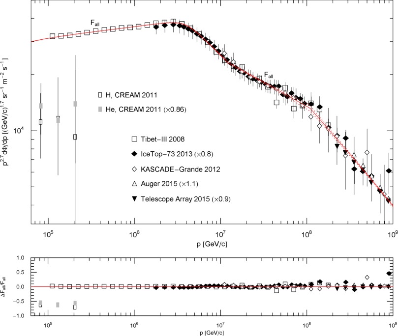
The high-energy spectral fit of the analytic flux density to the all-particle spectrum in the range is based on data points from Tibet-III [1], IceTop-73 [2] and [3], KASCADE-Grande [4], Auger [5] and Telescope Array [6]. The exponential decay of the flux density above 1010 GeV is caused by the Boltzmann factor; the decay exponent, defining the temperature of the relativistic non-equilibrium gas (ultra-relativistic in this region), is obtained from the spectral fit. The all-particle spectrum is an additive superposition of four spectral peaks which can iteratively be reconstructed from the multiplicative spectral kernel.
In the mildly relativistic low-energy regime , we approximate the all-particle flux by adding the flux densities of protons and helium nuclei, as heavier nuclei constitute only about one percent of the total flux in this interval. The proton and helium fluxes in the range are inferred from spectral fits to AMS-02 [7] and [8] and CREAM [9] data sets. The multiplicative spectral representation of the flux density allows us to perform the high- and low-energy fits separately, and it provides an analytic interpolation of the all-particle flux in the decade not yet covered by data points.
The spectral flux density used in the wideband fit of the all-particle spectrum is classical, admitting a partition function which can be assembled in relativistic phase space. We also sketch the quantization of the flux and number densities, partition function and thermodynamic variables, and find the conditions for the classical limit to apply. The factorizing flux density of the all-particle spectrum admits a decomposition into four partial fluxes which produce spectral peaks intersecting at the spectral breaks, and we calculate their thermodynamic parameters.
In Section 2, we introduce the flux densities employed in the spectral fits (performed in Section 5). Starting with the spectral number density of a free relativistic gas in stationary non-equilibrium, we derive the flux density as well as integral representations of the partition function and the thermodynamic variables of number count, internal energy, entropy and pressure. The deviation of the number density from the relativistic Maxwellian equilibrium density is quantified by its factorizing spectral kernel, a multiply broken power-law with parameters to be determined from spectral fits. In this way, we arrive at a product representation of the flux density suitable for wideband fits covering multiple spectral breaks.
In Section 3, we study the phase-space probability distribution defining the spectral number and flux densities. We obtain the phase-space representation of the thermodynamic variables and derive the entropy functional of the stationary non-equilibrium densities introduced in Section 2. The spectral densities discussed in Sections 2 and 3 are classical. In Section 4, we quantize these densities in Fermi and Bose statistics depending on the spin of the nuclei. At low fugacity, the quantum distributions become virtually undistinguishable from the classical densities. In Section 6.2, we give estimates of the fugacity of cosmic-ray nuclei, which turns out to be very small, so that the classical flux densities are uniformly applicable over the complete spectral range.
In Section 5, we perform spectral fits to the proton and helium fluxes in the interval as defined by AMS-02 and CREAM flux data. We use the analytic factorizing flux densities introduced in Section 2, which also admit extrapolation to lower energies. As the cosmic-ray flux in this interval consists almost entirely of hydrogen and helium nuclei, we obtain an approximation of the low-energy all-particle flux by adding the proton and helium flux densities. In the ultra-relativistic interval, where nuclear masses become negligible, we perform a fit to the all-particle spectrum covered by data sets from Tibet-III, IceTop-73, KASCADE-Grande, Auger, and Telescope Array. The spectrum in this interval shows several spectral breaks such as knee and ankle and two less pronounced breaks in their interconnecting slope as well as an ultra-high energy cutoff above 1010 GeV. The low-energy flux density obtained from the proton and helium spectra in the interval is extended to higher energies by iteratively adding factors to the low-energy spectral kernel which are defined by successive spectral breaks, as outlined in Appendix A. In this way, we obtain the flux density of the wideband spectrum ranging from 1 GeV to 1011 GeV.
In Section 6, we show that the all-particle spectrum admits an additive decomposition into four exponentially decaying spectral peaks with crossovers at the spectral breaks. The partial flux densities generating the peaks are iteratively extracted from the factorizing total flux density. We calculate the thermodynamic parameters of the all-particle flux and the partial fluxes, namely the specific densities of number count, internal energy and entropy as well as the pressure. In Section 7, we present our conclusions. In Appendix A, we explain wideband spectral fitting with factorizing flux densities.
2. Flux densities with factorizing spectral kernel
The spectral number density of a relativistic gas in stationary non-equilibrium reads [10] and [11]
where we have put ℏ=c=1. β=1/(kBT) denotes the temperature parameter, p is the momentum variable and s the spin degeneracy of the gas particles. The fugacity parameter α determines the normalization of the density, the fugacity being z=e−α. The all-particle cosmic-ray flux will be assembled with partial densities of type (2.1), with varying spin degeneracy and nuclear mass m, see Section 5.2. The spectral kernel h(p) defines a perturbation of the equilibrium phase-space probability, see Section 3, to be determined from spectral fits; the relativistic Maxwell equilibrium density is recovered by putting h(p)=1 in (2.1). The differential flux density per steradian based on number density (2.1) is
with momentum variable p in units of GeV/c and group velocity υ=dE/dp=p/E. The dispersion relation reads with Lorentz factor . In Section 5, we will employ the rescaled flux density
after restoring units. The spin degeneracy factor is s=2 for protons and s=1 for scalar bosons such as alpha particles. The scaling exponent κ in ( 2.3) can be freely chosen, as it does not affect least-squares fits, since the scale factor pκ drops out of the χ2 functional once the data points are rescaled with the same factor.
In order to minimize the χ2 functional, a good initial guess of the flux density is needed, uniformly valid over the complete spectral range. In a wideband fit extending over several energy decades, it is crucial to first locate the spectral breaks. The starting point, therefore, is to rescale the flux data so that the breaks become clearly visible in log-log plots. In the case of the all-particle cosmic-ray flux, this is achieved with a scaling exponent κ=2.7 in (2.3). The rescaling facilitates the systematic construction of an initial guess for the flux density, from spectral break to spectral break, covering a spectral range stretching over eleven orders in energy, as explained in Section 5.1 and Appendix A.
The spectral number and flux densities in (2.1) and (2.3) are related by
with c[m/s] and p[GeV/c]. The deviation of flux density ( 2.3) from thermal equilibrium is specified by a factorizing spectral kernel in the form of a multiply broken power law with smooth transitions,
where the amplitudes ck<ck+1 define the location of the spectral breaks, inferred from a spectral fit like the exponents γk > 0 and δk. Each factor in ( 2.6) represents a spectral break, and the factors are ordered by increasing amplitude. Wideband fits can iteratively be assembled by successively adding factors to the product (2.6), provided that the spectral breaks are sufficiently separated, ck<<ck+1, see Section 5.1. The number density (2.1) converges to the Maxwell equilibrium distribution in the non-relativistic limit, since h(p→0)=1.
To obtain integral representations of the thermodynamic variables, it is convenient to use a slightly more general distribution function than stated in (2.1),
which defines the partition function studied in Section 3; V is a volume factor. The parameters γ and δ drop out in variables obtained as derivatives of log Z at γ=1, δ=0. The number count N, internal energy U and pressure P read
The integration measure in (2.8)–(2.10) is the number density (2.1), coinciding with density (2.7) at γ=1, δ=0. The integral kernel of the pressure variable (2.10) is the product of momentum p , velocity and a geometric factor taking account of the incidence angles of the gas particles (incident upon an infinitesimal surface element). The entropy rescaled with the Boltzmann constant is obtained as
where log Z is taken at γ=1, δ=0. The fugacity parameter α can be extracted from the flux amplitude ( 2.4) and the temperature parameter β from the exponential cutoff in flux density ( 2.3). In Section 3, we will derive the entropy variable (2.11) from the phase-space probability density. The fourth term in (2.11) is the excess entropy
For the classical densities (2.1), this can be simplified by substituting the classical relation logZ=N according to (2.8). The entropy of the quantum distributions discussed in Section 4 is defined by (2.13), with number density dρ(p ) in the above integral representations replaced by the quantized counterpart. In equilibrium, h(p)=1, the excess entropy H vanishes and we can identify βPV=logZ(δ=0) via integration by parts.
3. Partition function and entropy
To derive the classical partition function defined by number density (2.1), we start with the n-particle phase-space measure
where the spatial d3qk integrations range over a volume V and the d3pk integrations over momentum space. (The normalization with (2π)3n is obtained by performing the classical limit in the quantized number densities derived in Section 4.) The n-particle probability density leading to number density ( 2.7) reads [13]
where Z is a normalization constant and bn(p) is the phase-space analogue to the exponential in (2.7). The spectral function h(p) defined in ( 2.6) quantifies the perturbation of the equilibrium phase-space probability. Density Pn(p) is independent of the space coordinates as there is no interaction potential included. We will ultimately put γ=1, δ=0 as in Section 2. The normalization condition is
where the summation is over the fluctuating particle number n. The factorial accounts for indistinguishability, and s is the spin degeneracy. In this way, we find the normalization constant Z in ( 3.2) as
The expectation value 〈n 〉 coincides with the number count N=logZ in (2.8), after evaluation of the factorizing integrals. The phase-space representation of internal energy, pressure and excess entropy in (2.9), (2.10) and (2.12) is obtained in like manner via differentiation of Z in ( 3.5),
are the random variables of energy, pressure and excess entropy in phase space. All derivatives are taken at γ=1, δ=0. The entropy variable is assembled as
where log Z and the probability density Pn(p) are taken at γ=1, δ=0. Substitution of the above averages into (3.11) leads to S in ( 2.13). The quantum analogue to the −kBPnlogPn phase-space representation of entropy is briefly discussed after (4.7).
4. Quantization of stationary non-equilibrium densities
The quantized version of the classical partition function Z in ( 3.5) is obtained by a trace calculation in fermionic (F) or bosonic (B) occupation number representation [14] and [15],
The particle number operator is , , where the are fermionic or bosonic creation/annihilation operators. The energy operator reads , the excess entropy is quantized as , and the pressure operator is . The Hermitian number operators are diagonal, . The fermionic occupation numbers nk attached to a wave vector k can take the values zero and one, whereas for bosons, the nk are non-negative integers. We employ box quantization, discretizing the wave vectors as k=2πn/L, so that k summations are taken over integer lattice points n, corresponding to periodic boundary conditions on a box of volume V=L3.
With these prerequisites, trace (4.1) can be evaluated in Fermi statistics as
Performing the thermodynamic continuum limit L → ∞ and taking into account the spin degeneracy, we can replace the summation in ( 4.5) by the integration sV∫d3k/(2π)3,
taken at γ=1, δ=0. For instance, density dρF/dk with s=2 applies to protons and dρB/dk with s=1 to 4He nuclei. The internal energy U=−(logZF,B),β, the excess entropy H/kB=−(logZF,B),γ and the pressure VP=−(logZF,B),δ are obtained from the quantized partition function (4.6) analogously to the classical case in (2.9), (2.10) and (2.12), and the total entropy S is assembled as in ( 2.13).
The quantized version of the phase-space representation of entropy in (3.11) is ; the counterpart to the phase-space probability density Pn(p) in (3.2) is the density operator , and the entropy operator is the counterpart to the entropy random variable sn in ( 3.12). The quantized partition function ZF,B(γ=1,δ=0) is stated in (4.1), and the operators , and are defined after (4.1). The excess entropy is determined by the spectral function h(p) in ( 2.6) which can be obtained from a spectral fit, see Section 5. specifies the deviation of from an equilibrium density operator. The counterpart to the phase-space normalization (3.4) is .
The fermionic/bosonic flux densities dΦF, B/dk read as in ( 2.2), with the classical density dρ/dp replaced by dρF, B/dk . (k=p since we have put ℏ=c=1.) To recover the classical limit (2.1) of the number densities dρF, B/dk, we only need to replace the factor 1/(eG(p) ± 1) in (4.7) by . The condition for the classical limit is thus e−G(p)<<1, which holds for cosmic-ray nuclei over the complete spectral range, as the fugacity z=e−α of the partial fluxes is very small, see the caption to Table 2. Therefore, we can use the classical number and flux densities in (2.1) and (2.2) to estimate the thermodynamic parameters of cosmic-ray fluxes, see Section 6.2.
5. Proton and helium fluxes and the all-particle energy spectrum
5.1. Product representation of spectral flux densities over multiple spectral breaks
The spectral fits are performed with the rescaled flux density (2.3), F=pκdΦ/dp,
where is the factorizing spectral kernel introduced in (2.6), a multiply broken power-law with smooth transitions at the spectral breaks. We use the scaling exponent κ=2.7 to make spectral breaks visible in log-log plots of the all-particle spectrum covering the complete interval, see also the remarks after (2.4). Usually (but not always) the exponents δk of the spectral kernel have alternating signs, assuming that the factors of h(p ) are ordered by increasing amplitude, ck<ck+1. The ck define the location of the spectral breaks, and the exponents γk together with the sign of δk determine the slopes of the spectral curve between the breaks. A moderate or large |δk| leads to a smoothing of the spectral break at p ≈ ck, that is, to a gradual change of the slope in the vicinity of p ≈ ck. A |δk| close to zero results in a sudden break in the spectral curve, appearing as edge joining two nearly straight (approximately power-law) slopes in log-log plots. This is illustrated by the spectral breaks visible in the figures and the numerical value of the exponents δk attached to the respective break points ck listed in Table 1. The product representation of h(p ) is efficient if the spectral breaks are widely separated, ck≪ck+1. In this case, one can perform an iterative fit over an extended spectral range as outlined in Appendix A. Finally, the nuclear mass in (5.1) becomes negligible if m2/p2 ≪ 1. That is, at energies above 104 GeV, in the ultra-relativistic regime, the mass squares in (5.1) can be dropped even for iron nuclei.
Table 1.
Fitting parameters of the proton and helium spectra in Figs. 1 and 2 and of the all-particle spectrum in Fig. 3, Fig. 4, Fig. 5, Fig. 6, Fig. 7 and Fig. 8. The spectral fits are performed with the proton and helium flux densities FH, low and FHe, low in (5.3) and the all-particle flux density Fall in (5.4). The amplitudes ck in the power-law factors of Fall define the location of the spectral breaks, and the exponents γk and δk determine the slopes and curvature of the spectral curves depicted in the figures, as pointed out after ( 5.1). (c4 is the knee, c6 the second knee and c7 the ankle, see Fig. 8.) The temperature parameter kBT is extracted from the exponential spectral cutoff of the all-particle flux density ( 5.4); kB denotes the Boltzmann constant. AΦ,H and AΦ,He are the amplitudes of the low-energy proton and helium flux densities (5.3).
In view of the phase-space reconstruction of the thermodynamic variables in Section 3 and the quantization of the partition function in Section 4, the momentum parametrization of flux density (5.1) is the natural choice. We briefly point out the conversion of the momentum parametrization to a parametrization by kinetic energy per nucleon as well as to a rigidity parametrization [16], both often used in observational papers. We write the energy of the nucleus as E=nEk+m=mγL, with Lorentz factor , where n is the number of nucleons, Ek the kinetic energy per nucleon and m the mass of the nucleus. The dispersion relation is . We use GeV units for energy, writing p[GeV/c ] (momentum per nucleus) in the figures. The conversion of momentum plots to plots parametrized by kinetic energy per nucleon Ek[GeV/n] is thus performed with and
where F(p)=pκdΦ/dp as in (5.1). We will put n=1 for hydrogen and n=4 for helium, assuming 1H and 4He isotopes [8] and [17]. At high energy, we can neglect the rest mass (using the 0th order of an m/(nEk) expansion of (5.2)), and approximate p∼nEk, . The conversion of the momentum parametrization in (5.1) to a parametrization by rigidity R=cp/(Ze) (where e is the electron charge, taken positive, and Z the charge number of the nuclei) is performed with p[GeV/c]=ZR[GV] and RκdΦ/dR=Z1−κF(ZR). For protons, momentum plots in p[GeV/c] thus coincide with rigidity R[GV] plots.
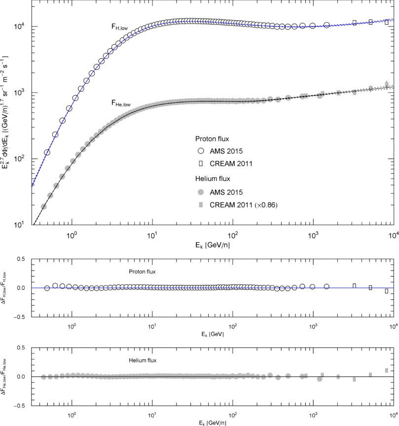
Fig. 1 shows spectral fits to the AMS-02 hydrogen and helium fluxes, with CREAM data points added, in the low-energy interval from 1 GeV to 104 GeV. For protons, the fit is performed with flux density
Proton and helium flux densities in the low-energy regime . Data points from AMS-02 [7] and [8] and CREAM [9]. The hydrogen and helium spectra are fitted with the flux densities FH, low(p) and FHe, low(p) in ( 5.3) (solid curves) and parameters listed in Table 1. The helium CREAM points are rescaled by a factor of 0.86 to obtain a smooth continuation of the AMS-02 data set. The error bands defined by the dotted curves indicate the 1σ confidence limits of the least-squares fits, χ2(H)/dof ≈ 15.1/68, χ2(He)/dof ≈ 12.2/66; the residuals are depicted in the lower panels. By adding the spectral curves, FH,low+FHe,low, we obtain an approximation of the all-particle spectrum, as heavier nuclei contribute only about one percent to the total flux at energies below 104 GeV. The specific number densities of protons and helium nuclei below 104 GeV are 1.07×10⁻⁴/m3 and 1.6×10⁻⁵/m3, respectively, obtained by truncating the integral representation of the number density in (6.8) at 104 GeV and substituting the low-energy flux limits (5.3). The spectral curve of the proton flux FH, low remains unchanged in rigidity parametrization, if the coordinate labels are replaced by R [GV] and R2.7dΦ/dR[GV1.7sr−1m−2s−1], see after (5.2); this is not the case for the helium flux, as the charge number differs from one.
where is the proton mass and κ=2.7 the rescaling exponent, see (2.3) and after (5.1). As there is no spectral cutoff visible in the low-energy data sets, we drop the exponential in (5.1), assuming a sufficiently high temperature so that below 104 GeV. The fitting parameters, labeled by a subscript H in (5.3), are listed in Table 1. The same density (5.3) with subscript H replaced by He is employed in the spectral fit of the low-energy helium flux FHe, low. We use as helium mass assuming alpha particles. The parameters AΦ,He, c1He, etc. of the helium fit in Fig. 1 are also recorded in Table 1. We obtain an approximation of the low-energy all-particle flux density in the interval by adding the proton and helium fits, Fall,low∼FH,low+FHe,low, see Fig. 1, since heavier nuclei contribute only about one percent to the total flux in this energy range. In Fig. 2, the momentum parametrization of the proton and helium fluxes is converted to a parametrization by kinetic energy per nucleon by means of (5.2).
Fig. 2.
Spectral densities of the low-energy hydrogen and helium fluxes, parametrized by kinetic energy per nucleon. Data points from AMS-02 [7] and [8] and CREAM [9]. The spectral curves and flux points in Fig. 1 are converted from momentum representation to Ek (kinetic energy per nucleon) representation by way of transformation (5.2), assuming 1H and 4He isotopes. As we consider a free relativistic gas of cosmic-ray nuclei rather than nucleons, a flux parametrization by momentum per nucleus has been adopted in this paper except for this figure; also see the end of Section 5.1 for flux parametrization in the ultra-relativistic regime above 104 GeV.
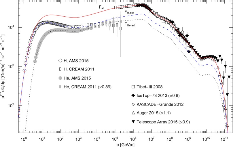
In Fig. 3, we perform a spectral fit to the all-particle flux above 105 GeV. To this end, we extend the low-energy flux Fall, low by adding power-law factors defined by successive spectral breaks as explained after (5.1):
Wideband spectral map of the all-particle flux. Low-energy data points from AMS-02 [7] and [8] and CREAM [9]. High-energy data from Tibet-III (QGSJET+PD) [1], IceTop-73 (rescaled by a factor of 0.8) [2] and [3], KASCADE-Grande [4], Auger (rescaled by 1.1) [5] and Telescope Array (SD and FD Mono, rescaled by 0.9) [6]. The rescaling is required to make the data sets compatible in overlapping intervals so that they define a continuous spectral curve. The solid curve depicts the all-particle flux Fall defined by flux density (5.4) with parameters in Table 1. Below 104 GeV, Fall can be approximated by adding the low-energy proton and helium fluxes in Fig. 1, Fall∼FH,low+FHe,low, as pointed out after (5.3). Above 105 GeV, Fall is inferred from a least-squares fit to the high-energy flux points as explained after (5.4), with χ2/dof ≈ 223/101; also see the close-ups in Fig. 5, Fig. 6 and Fig. 7. The dashed and dotted curves depict extensions of the low-energy proton and helium fluxes in Fig. 1 defined by the partial fluxes FH, ext and FHe, ext in (5.5), both of which contain admixtures of heavier nuclei and add up to the total all-particle flux density Fall=FH,ext+FHe,ext of the wideband spectrum ranging from 1 GeV to 1011 GeV. These analytic flux densities also extrapolate the spectrum to energies below 1 GeV, as required in the integral representations (6.8)–(6.11) of the thermodynamic variables.
The parameters of the high-energy fit in the interval are (ck, γk, δk), k=3,…,7 and the cutoff temperature kBT defining the decay exponent β=1/kBT, see Table 1. The low-energy proton and helium fluxes FH, low and FHe, low are considered input obtained from the fits in Fig. 1. The factors in (5.4) are ordered by increasing spectral break, 104<<ck<<ck+1<<kBT, see Table 1, so that Fall approximates Fall, low below 104 GeV. In the χ2 functional of Fall(p), the parameters defining the densities FH, low and FHe, low (labeled with an H or He subscript in (5.3) and Table 1) are kept constant at the values inferred from the above described fits of the hydrogen and helium spectra. The high-energy flux points included in χ2 stem from Tibet-III [1], IceTop-73 [2] and [3], KASCADE-Grande [4], Auger [5] and Telescope Array [6], see Fig. 3. The sixteen parameters varied in the least-squares fit of Fall(p) are listed in Table 1 (without an H or He subscript). To find the minimum of this χ2, it is essential to have a good initial guess of the flux density; an iterative method to find this is sketched in Appendix A. The flux density Fall defined in (5.3) and (5.4) with parameters in Table 1 reproduces the all-particle energy spectrum in the range as depicted in Fig. 3. This analytic density also provides an extrapolation of the spectrum to energies below 1 GeV as well as an interpolation in the range not yet covered by data points, see the close-up in Fig. 4.
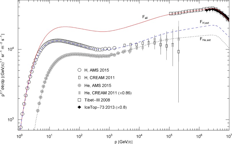
Fig. 4.
Crossover from the low- to the high-energy regime of the all-particle spectrum. This is a close-up of Fig. 3. The partial fluxes FH, ext and FHe, ext (dashed and dotted curves) are extensions of the low-energy spectral fits FH, low and FHe, low of the proton and helium spectra in Fig. 1, see (5.5) and the caption to Fig. 3. In the decade, the partial fluxes FH, ext and FHe, ext start to deviate from the depicted CREAM flux points due to admixtures of heavier nuclei, see also the remarks after (5.6). (Therefore, in the χ2 functionals of the low-energy fits in Fig. 1, we only included the first three hydrogen CREAM points and the first five helium CREAM points, respectively.) The all-particle flux density Fall=FH,ext+FHe,ext (solid curve) is the continuation of the low-energy flux FH,low+FHe,low in Fig. 1 to ultra-relativistic energies above 104 GeV; the analytic representation thereof is given in (5.4) and (5.5). A soft spectral break emerges
at c3 ≈ 6.9 × 10⁴ GeV, see Table 1.
At energies below 10 GeV, the proton and helium spectra become time dependent due to solar modulations as exemplified by the BESS-Polar spectra [18]. This time dependence can be accommodated in an adiabatic time variation of the fitting parameters (c1H, γ1H, δ1H) and (c1He, γ1He, δ1He) (which define the first spectral break of the proton and helium fluxes causing the broad peaks in Fig. 1, see (5.3) and Table 1), resulting in a quasi-stationary flux density (5.4). In this paper, we use time-averaged spectra and stationary spectral densities to model the proton and helium fluxes.
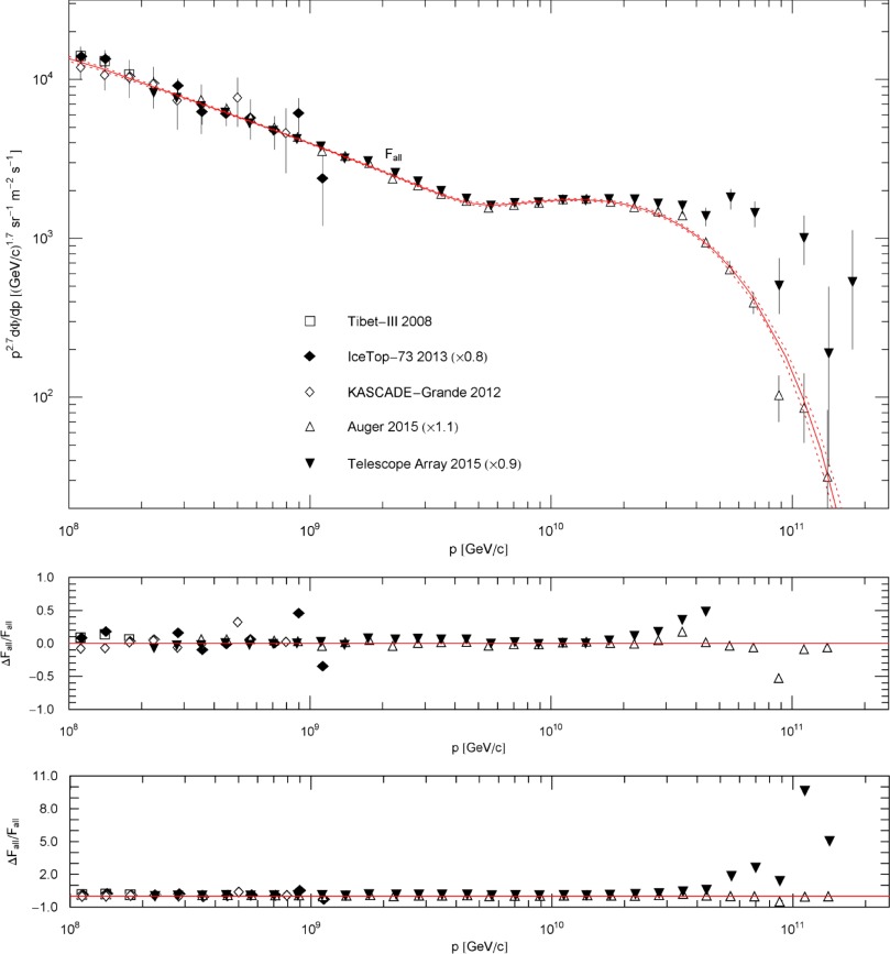
The fine-structure of the all-particle spectrum in the interval is illustrated by the close-ups in Fig. 5, Fig. 6 and Fig. 7, the latter two extending over four energy decades each. Between the knee c4 and the ankle c7 (listed in Table 1), there are two soft spectral breaks at and , which are clearly visible in Fig. 6 and accounted for by the respective factors in flux density (5.4). A close-up of the exponential spectral cutoff generated by the Boltzmann factor in the flux density is shown in Fig. 7. The Telescope Array flux points above 2 × 10¹⁰ GeV have not been included in the fit, as they substantially deviate from the Auger flux, which decays exponentially and allows us to extract the temperature parameter. The decay indicated by the Telescope Array points is less pronounced and may even turn out to be subexponential, of Weibull type for instance, with the Boltzmann factor in (5.4) replaced by exp(−ρ(βp)), the exponent 0 < ρ < 1 being an additional fitting parameter.
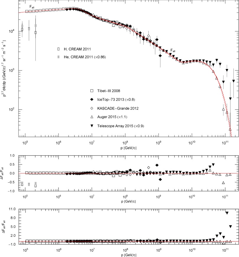
Fig. 5.
High-energy spectral fit to the all-particle flux in the interval, a close-up of the wideband spectrum in Fig. 3. Data points as listed in the caption of Fig. 3. The least-squares fit Fall (solid curve, χ2/dof ≈ 223/101) is performed with flux density (5.4), the fitting parameters are recorded in Table 1. In this ultra-relativistic regime, the coordinate labels can be replaced by E [GeV] (energy per nucleus) and E2.7dΦ/dE[GeV1.7sr−1m−2s−1], as the nuclear rest mass drops out of the dispersion relation. The dotted curves indicate the 1σ error band (better visible in the close-ups of Figs. 6 and 7). The last ten Telescope Array points depicted in the figure have not been included in the fit, see the remarks at the end of Section 5.1 and the caption to Fig. 7. The residuals are shown in the second and third panel. The latter includes the residuals of all Telescope Array points except the last one (with ΔFall/Fall ≈ 63.5), which is off the scale due to the rapid exponential decay of Fall. The second panel is a close-up of the third.
Close-up of the high-energy all-particle spectrum in Fig. 5. Data points as in Fig. 3. The solid curve Fall depicts flux density (5.4) with parameters in Table 1, the dotted curves define the 1σ error band. Residuals are shown in the lower panel. The knee is defined by the spectral break at , see also (5.4) and Table 1, and is followed by two less pronounced but still clearly visible breaks at and in the slope joining knee and ankle, the latter is shown in Fig. 7.
Decaying spectral tail of the all-particle spectrum. Close-up of Fig. 5, data points as in Fig. 3; the depicted ten highest energy points of the Telescope Array have not been included in the χ2 fit, as they are not compatible with the Auger data. The latter define an exponential spectral cutoff, whereas the Telescope Array points suggest subexponential Weibull spectral decay [31], [32], [33] and [34]. The caption to Fig. 5 applies regarding the flux density Fall (solid curve). The 1σ error band is indicated by the dotted curves. The ankle is the spectral break at , see Table 1. The exponential spectral decay is caused by the ultra-relativistic Boltzmann factor e−p/(kBT) of flux density (5.4) with cutoff temperature kBT ≈ 2.5 × 10¹⁰ GeV. The residuals are plotted in the two lower panels at different scales.
Above 104 GeV, we can identify E ∼ p, as the nuclear mass drops out of the dispersion relation, see after ( 2.2). Therefore, the plots in Fig. 5, Fig. 6 and Fig. 7 do not change in energy parametrization, that is, the coordinate labels can be replaced by E [GeV] and E2.7dΦ/dE[GeV1.7sr−1m−2s−1] in this ultra-relativistic regime. Here, E is the energy per nucleus, not to be confused with Ek labeling Fig. 2, which denotes energy (with nuclear rest mass subtracted) per nucleon, see (5.2).
5.2. Decomposition of the all-particle spectrum into partial fluxes
The all-particle flux density Fall in (5.4) is the superposition of two partial fluxes of type (5.1), Fall=FH,ext+FHe,ext, which are extensions of the low-energy proton and helium fluxes FH, low and FHe, low in (5.3):
and the helium extension FHe, ext(p) is obtained by replacing the subscript H by He. These partial fluxes are depicted in Figs. 3 and 4 as dashed and dotted curves. The factors in (5.5) defined by the break energies c1H, c2H and ck, k=3,⋯,7, constitute the spectral kernel hH, ext of FH, ext, see (5.1),
and analogously for hHe, ext. The numeration of the factors is by increasing spectral break, c1H<<c2H<<ck<<ck+1. The exponential in (5.5) corresponds to , β=1/kBT, in (5.1); since the cutoff temperature kBT is very high, see Table 1, we have dropped the mass square in the exponent. In the first ratio in (5.5), the nuclear mass is essential at low p, in the mildly relativistic regime.
The partial fluxes FH, ext and FHe, ext fit the hydrogen and helium spectra in the low energy range , where they approximate the flux limits (5.3). At higher energies, in the range, there are admixtures of heavier nuclei to both components, as their sum FH,ext+FHe,ext constitutes the flux Fall in (5.4) obtained from a fit to the all-particle spectrum. These admixtures of intermediate and heavy nuclei can even dwarf the hydrogen and helium contributions to the all particle flux FH,ext+FHe,ext over sections of the high-energy range, see the remarks after (6.7) and Refs. [19], [20], [21], [22] and [23]. The CREAM flux points define the proton and helium spectra in the interval, although with rather large error bars, see Fig. 4. Comparing these points to the flux extensions FH, ext and FHe, ext, there is already a small contribution from heavier nuclei noticeable in this interval, especially in the proton extension FH, ext.
We have split the all-particle flux density (5.4) into two partial fluxes, one depending on the hydrogen mass and one on the helium mass, see (5.5). The masses of heavier nuclei contributing to the flux densities FH, ext and FHe, ext do not enter, as the all-particle spectrum in the low-energy range essentially consists of protons and helium and, at high energies above 104 GeV, the rest masses are negligible, since the squared mass-energy ratio m2/p2 is very small even for iron nuclei. Above 104 GeV, the momentum variable can be identified with energy for the same reason. In Section 6, we will use the partial fluxes FH, ext and FHe, ext to decompose the all-particle flux Fall into a series of spectral peaks and to estimate their thermodynamic parameters.
6. All-particle spectrum as additive superposition of spectral peaks
6.1. Partial flux densities defined by spectral breaks
We start by splitting the factorizing flux density FH, ext in (5.5) into partial fluxes FH, ext,i generating four consecutive, exponentially decaying spectral peaks, . The decay exponent of FH, ext,i is denoted by βiH, and the peaks are ordered by decreasing decay exponent, β1H ≥ β2H ≥ β3H ≥ β4H. These exponents are free parameters, except for β4H which coincides with the temperature parameter of the all-particle flux, β4H=β=1/(kBT), inferred from the wideband fit. The exponents will be specified in (6.7) by identifying them with spectral breaks.
The partial fluxes constituting the hydrogen extension FH, ext in (5.5) are obtained iteratively. The flux density FH, ext,1 generating the first peak is found by dropping all numerators of FH, ext defined by spectral breaks, namely the factors
The partial fluxes defining the second, third and fourth peak are obtained by successively restoring the numerators (6.1), replacing the decay exponents βiH→β(i+1)H and subtracting the preceding peaks:
The subtraction of the preceding peaks does not violate positivity, as the second identities in (6.4)–(6.6) show, since the exponents defining the factors fi=2,3,4 in (6.1) are positive and the decay exponents satisfy βiH≥β(i+1)H. By adding the four fluxes FH, ext,i defined in (6.2) and (6.4)–(6.6), we recover flux density FH, ext in (5.5), provided that the smallest decay exponent β4H is identified with the temperature parameter β of FH, ext; the decay exponents of the first three peaks drop out in .
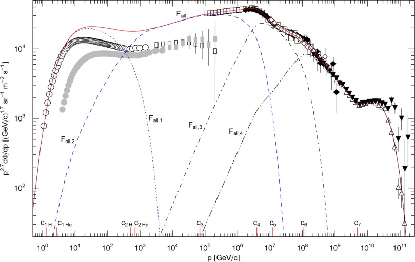
The decomposition of the helium flux extension into spectral peaks is performed analogously, ; we just need to replace the subscript H by He in the flux densities (6.2) and (6.4)–(6.6) and in the factors f1, 2 defined in (6.1) and (6.3). The four spectral peaks Fall,i in Fig. 8 constituting the all-particle flux are obtained by adding the corresponding peaks of the extended hydrogen and helium components, Fall,i=FH,ext,i+FHe,ext,i, see the beginning of Section 5.2.
Fig. 8.
All-particle energy spectrum as additive superposition of spectral peaks. Data points as in Fig. 3. The solid curve Fall is the χ2 fit of the all-particle flux density (5.4), see also the caption to Fig. 3. The iterative decomposition of this flux density into spectral peaks is explained in Section 6.1. The four strongly overlapping peaks Fall,i (dotted/dashed curves) add up to the all-particle flux . The spectral breaks ck listed in Table 1 are indicated on the abscissa. All four peaks terminate in exponential decay, see (6.7): Fall,2 is exponentially cut at the knee c4 and Fall,3 at the second knee c6; the cutoff of the low-energy peak Fall,1 is defined by the spectral breaks c2H and c2He in the hydrogen and helium components of the all-particle flux. The double peak Fall,4 coalesces with the exponentially decaying all-particle flux above the ankle c7. The thermodynamic parameters of the total flux Fall and the partial fluxes Fall,i generating the peaks are recorded in Table 2.
The exponential decay of the fourth peak Fall,4, which is actually a double peak centered at the ankle c7, is determined by the cutoff temperature of the all-particle flux, β4H=β4He=1/(kBT), see Table 1. The knee c4 and the second knee c6 emerge at the intersections of overlapping fluxes, Fall,2, Fall,3 and Fall,3, Fall,4, respectively, see Fig. 8.
The first peak Fall,1 in Fig. 8 located below 104 GeV has a light mass composition, as the all-particle spectrum below 104 GeV consists predominantly of proton and helium nuclei. The second peak Fall,2 in Fig. 8 (which is exponentially cut at the knee c4) has also a light composition below 104 GeV for the same reason. Above 104 GeV, the all-particle spectrum increasingly deviates from the combined CREAM proton and helium spectra, due to admixtures of heavier nuclei, see Section 5.2 and Fig. 4. Composition studies with Tibet-III indicate that the light component accounts for less than 30% of the all-particle flux in the knee region [19] and [20]. This suggests that the second peak Fall,2 has an increasingly heavy composition above 104 GeV, containing at least intermediate-mass nitrogen-like nuclei.
Above the knee, the IceCube Collaboration derives a mean log mass which increases in the interval between 5 × 10⁶ GeV and 3 × 10⁸ GeV where it reaches a plateau and starts to decrease [3]. Composition studies with the Yakutsk array in the range also indicate a maximum of the mean log mass at around 108 GeV followed by a substantial decrease in the subsequent decade [21]. A heavy iron-like composition at the second knee around 108 GeV has also been found by the KASCADE-Grande Collaboration [22] and [23]. Above 109 GeV, a light composition is inferred with the Telescope Array [6], whereas a mixed composition, mainly light to intermediate, is suggested by the Auger Collaboration [24]. Accordingly, the fourth peak Fall,4 in Fig. 8 has a light or light-to-intermediate composition, whereas the third peak Fall,3, which covers the knee c4 and is exponentially cut at the second knee c6, has presumably a heavy composition.
Models of diffusive shock acceleration in supernova remnants (SNRs) suggest that protons in SNR shocks can reach energies up to the knee at c4 ∼ 4 × 10⁶ GeV [25] and [26]. As the maximum energy obtainable by shock acceleration scales with the atomic charge number, the iron component can thus extend to energies of around 108 GeV, reaching the second knee c6. This is consistent with the above quoted composition studies, which suggest a heavy component extending to the second knee and declining above [21]. This heavy component is manifested as spectral peak Fall,3 in Fig. 8. The existence of high-energy ( ∼ 105 GeV) protons in SNRs is also supported by the TeV γ-ray spectra of several SNRs (enumerated in Refs. [27] and [28]) which could stem from hadronic γ-ray production by pion decay, the pions being generated in collisions of high-energy protons with nuclei. The first three peaks in Fig. 8 could thus be produced by shock acceleration in SNRs. Another possible source mechanism is one-shot acceleration in the induced electric fields of pulsars [29].
The fourth peak Fall,4 in Fig. 8 constituting the ultra-high energy component of the all-particle spectrum is a double peak which, above the ankle c7, coincides with the all-particle flux. Assuming an extragalactic origin of this peak (possible sources could be shock acceleration in active galactic nuclei, also γ-ray bursts or decaying super-massive particles [25]) and a proton-dominated composition, the exponential cutoff of this peak can be explained by scattering of protons by cosmic microwave background photons (energy loss via pion production, GZK cutoff [25]). In the case of a light-to-intermediate mass composition, the cutoff could be caused by acceleration limits of the sources. The double-peak structure of Fall,4 could be carved out by attenuation effects such as electron-positron pair production, again by scattering of protons by microwave photons, or photo-disintegration of heavier nuclei, also caused by interaction with microwave photons or the extragalactic background light [30].
The cutoff of the third peak Fall,3 also affects the shape of the fourth peak because of the subtraction in (6.6). If the peak Fall,3 is cut off at the ankle, β3H=β3He=1/c7, instead of at the second knee c6 as in (6.7), then the double peak Fall,4 in Fig. 8 shrinks to a single peak with its maximum located above the ankle. The latter then emerges at the intersection of a broad Galactic peak Fall,3 and a small extragalactic peak Fall,4. However, a heavy mass component Fall,3 extending to the ankle is at odds with the mentioned composition studies (e.g. Ref. [21]), which indicate a cutoff of the heavy component at the second knee as shown in Fig. 8.
The multiplicative flux representation (5.4) is more efficient than an additive superposition of spectral peaks when performing wideband fits, especially if the source mechanisms are uncertain and the peaks are substantially overlapping as in Fig. 8. The iterative decomposition of the wideband spectrum into spectral peaks is subsequently carried out without invoking approximations.
6.2. Thermodynamic parameters of cosmic-ray fluxes
We will calculate the specific number and energy densities N and U, the excess entropy density H and the pressure P, based on the integral representations ( 2.8)–(2.10) and (2.12). (The specific densities are obtained by dropping the volume factors there.) By making use of the flux representation of the spectral number density in (2.5), we find
with c [m/s]. The specific density of the total entropy is assembled as S/kB=(α+1)N+βU+H/kB, see (2.13), with fugacity and temperature parameters α=log(1.573×1053s/AΦ) and β=1/kBT[GeV], where AΦ is the flux amplitude and s the spin degeneracy of the gas particles as in ( 2.4).
We denote the specific densities and the pressure of the extended hydrogen flux FH, ext in (5.5) by NH, ext, UH, ext, HH, ext and PH, ext, and calculate these quantities with FH, ext and hH, ext in (5.6) substituted into the integral representations (6.8)–(6.11). The total entropy density of this partial flux is SH,ext/kB=(αH+1)NH,ext+βUH,ext+HH,ext/kB, with fugacity parameter αH=log(1.573×1053sH/AΦ,H), spin degeneracy sH=2 and flux amplitude AΦ,H listed in Table 1.
The thermodynamic parameters of the extended helium flux FHe, ext are obtained analogously and denoted by NHe, ext, UHe, ext, HHe, ext, PHe, ext and SHe, ext; the fugacity parameter αHe is calculated with spin degeneracy sHe=1 and amplitude AΦ,He in Table 1. The specific densities Nall, Uall, Hall, Sall and the pressure Pall of the all-particle flux Fall in (5.4) are listed in the first row of Table 2, obtained by adding the respective densities and pressure variables of the partial fluxes FH, ext and FHe, ext, e.g. Nall=NH,ext+NHe,ext.
Table 2.
Thermodynamic parameters of the all-particle flux Fall and the partial fluxes Fall,i in Fig. 8. N denotes the specific number density, U the specific internal energy density, H/kB and S/kB are the specific densities of excess entropy and total entropy (rescaled with the Boltzmann constant) and P is the pressure, see Section 6.2. In the first row, these quantities are listed for the all-particle flux Fall; their calculation is explained after (6.11). The total entropy density S/kB of the all-particle flux is assembled with the extended hydrogen and helium fluxes FH, ext and FHe, ext in (5.5) and their fugacity parameters αH=114.1 and αHe=117.8. As the fugacity is very small, zH,He=exp(−αH,He), the classical flux densities used in the spectral fits are applicable over the complete spectral range, see the end of Section 4. Also recorded are the thermodynamic parameters of the partial fluxes Fall,i generating the four spectral peaks in Fig. 8; these parameters are assembled as outlined after (6.12) and add up to the corresponding quantities of the all-particle flux Fall.
Also recorded in Table 2 are the specific densities Nall,i, Uall,i, Hall,i, Sall,i and the pressure Pall,i of the partial fluxes generating the spectral peaks Fall,i, i=1,⋯,4, depicted in Fig. 8. To assemble these variables, we first express the partial fluxes FH, ext,i in (6.2) and (6.4)–(6.6) by flux densities which are structured as in (2.3) and (2.6): FiH=f0hiHe−βiHp, with spectral kernels
The factors fi=0,…,4 are defined in (6.1)–(6.3) and the exponents βiH in (6.7). The four partial fluxes FH,ext,i=FiH−F(i−1)H (with F0H=0) add up to the total flux FH, ext in (5.5), see also after (6.6).
We write N(FiH), U(FiH), H(FiH, hiH) and P(FiH) for the specific densities (6.8)–(6.11), with FiH and hiH substituted for the flux F and the spectral kernel h in the integrands. The specific number density NH, ext,i of the partial flux FH, ext,i is calculated as NH,ext,i=N(FiH)−N(F(i−1)H), and analogously UH, ext,i, HH, ext,i and PH, ext,i. The specific total entropy density of FH, ext,i reads SH,ext,i=S(FiH)−S(F(i−1)H) with
The fugacity parameter αH is calculated as explained after (6.11), also see the caption to Table 2. The specific number densities of the partial fluxes FH, ext,i add up to the number density NH, ext of the total flux FH, ext already calculated after (6.11), , and analogously for energy, excess entropy, total entropy and pressure.
The foregoing derivations also apply to the extended helium flux FHe, ext, with subscript H replaced by He. The specific densities Nall,i, Uall,i, Hall,i, Sall,i and the pressure Pall,i of the partial fluxes Fall,i defining the spectral peaks in Fig. 8 are found by adding the corresponding densities of the extended hydrogen and helium components, Nall,i=NH,ext,i+NHe,ext,i, etc. The all-particle flux Fall is the sum of the partial fluxes Fall,i, as pointed out after (6.6). Accordingly, the specific number density Nall of the all-particle flux calculated after (6.11) can also be obtained by adding the number densities Nall,i of the four spectral peaks Fall,i in Fig. 8, see Table 2, and this holds as well for the specific energy and entropy densities and the pressure.
7. Conclusion
Cosmic-ray nuclei constitute a relativistic multi-component gas in stationary non-equilibrium. We have found the partition function of this gas, defined by a spectral flux density which accurately reproduces the spectral range currently accessible, from 1 GeV to 1011 GeV. Spectral maps of the all-particle energy spectrum in log-log representation exhibit, besides knee and ankle, several weaker, widely spaced spectral breaks. In the least-squares fits, we used a multiplicative spectral representation of the flux density, each factor being determined by a spectral break. The wideband fit can iteratively be performed over an extended energy range by adding factors to the spectral kernel of the flux density, which is a multiply broken power-law function defined by successive spectral breaks, see (2.6) and Section 5.1. The factorizing all-particle flux density admits an additive decomposition into four partial fluxes, each of them generating a spectral peak which is exponentially cut off at a spectral break.
We have chosen to model cosmic-ray nuclei as stationary non-equilibrium system and to extract the number density and partition function thereof from available spectra. In this way, we can avoid making specific assumptions on source distributions and interaction mechanisms producing the spectral peaks, which otherwise would have to be quantified in models based on kinetic equations. Instead, the spectral peaks constituting the wideband spectrum are iteratively reconstructed from the fitted flux density. The qualitative mass composition of the peaks and possible Galactic and cosmological source mechanisms are briefly discussed at the end of Section 6.1.
The spectral number density (2.1) employed in the spectral fits can be traced back to the phase-space probability distribution studied in Section 3. Once this distribution is known, one can assemble the partition function of the relativistic nuclei and calculate the thermodynamic variables, as done in Sections 3 and 6.2. We quantized the classical spectral number density in Fermi and Bose statistics, depending on the nuclear spin, see (4.7). In either case, the classical density (2.1) approximates the quantum density in the limit of vanishing fugacity. As the fugacity of cosmic-ray fluxes is extremely small, see the caption to Table 2, the classical formalism of Section 2 applies over the complete spectral range.
Figs. 1 and 2 depict spectral fits to the AMS-02 [7] and [8] and CREAM [9] proton and helium spectra. Both of these low-energy spectra consist of a peak followed by a trough and a slightly increasing slope. The peak and trough are treated as spectral breaks defining the factorizing kernel of the flux density employed in the fits, see (5.3) and Table 1. By adding the proton and helium flux densities, we obtained an approximation to the all-particle flux in the interval, since heavier nuclei contribute only a negligible fraction, roughly one percent of the all-particle flux, in this interval.
The low-energy flux density is then iteratively extended to higher energies by fitting the all-particle spectrum defined by the Tibet-III [1], IceTop-73 [2] and [3], KASCADE-Grande [4], Auger [5] and Telescope Array [6] data sets, see Fig. 3. The high-energy fit in the interval is performed with the analytic flux density defined in (5.4) and Table 1, which is a multiply broken power-law function with smooth transitions at the spectral breaks and an exponential ultra-high energy cutoff by the Boltzmann factor. This flux density also provides an interpolation of the all-particle spectrum in the interval. The crossover from the low- to the high-energy spectrum is shown in Fig. 4. The spectral breaks of the high-energy component are visible in Fig. 5, Fig. 6 and Fig. 7 (which are close-ups of the wideband spectrum in Fig. 3), in particular the two soft breaks between knee and ankle resulting in a slight shift of the spectral slope, see Fig. 6. The exponentially decaying spectral tail is shown in Fig. 7; the temperature parameter in the Boltzmann factor of this stationary non-equilibrium gas of relativistic nuclei is inferred from the spectral fit. The all-particle flux density of the wideband spectrum is an additive superposition of four strongly overlapping spectral peaks with crossovers at the spectral breaks as depicted in Fig. 8. The iterative flux decomposition into exponentially decaying spectral peaks is explained in Section 6.1. The thermodynamic parameters of the total flux and of the partial fluxes constituting the spectral peaks are calculated in Section 6.2 and recorded in Table 2.
Appendix A. Iterative wideband fitting
The χ2 functional of flux density Fall(p) in ( 5.4) depends on sixteen parameters, (ck, γk, δk), k=3,…,7, and kBT , which have to be varied simultaneously to find the minimum. Therefore, a good initial guess for the flux density is required, valid over the complete spectral range . As the spectral breaks are widely separated, ck<<ck+1, see Table 1 and Fig. 3, Fig. 4, Fig. 5, Fig. 6 and Fig. 7, it is possible to iteratively find an initial guess for Fall(p) by varying six parameters in each step (seven in the last one).
In the analytic flux density Fall(p) in ( 5.4), we drop the exponential and the three factors defined by the last three breaks (ck, γk, δk), k=5,6,7, and denote this density by Fall(p; 3, 4). The χ2(3, 4) functional of Fall(p; 3, 4) is defined by using the Tibet-III and IceTop-73 flux points with energies below the spectral break at c5 ≈ 1.2 × 10⁷ GeV, see Fig. 6. (The precise location of the spectral breaks ck, k=3,…,7, is not known at this stage, but can be estimated by plotting the properly rescaled flux points, see the remark after (2.4) and Fig. 8.) By minimizing χ2(3, 4), we obtain preliminary values for the parameters (ck, γk, δk), k=3,4. This is the first step of the iteration.
The second step is based on density Fall(p ; 3; 4, 5) defined in like manner by dropping the last two factors indexed k=6,7 and the exponential in (5.4). For the parameters (c3, γ3, δ3), we substitute the values obtained from the previous χ2(3, 4) fit. The χ2(4, 5) functional of Fall(p; 3; 4, 5) thus depends on the parameters (ck, γk, δk), k=4,5. The flux points included in χ2(4, 5) have energies up to the spectral break c6 ≈ 1.1 × 10⁸ GeV, see Fig. 6. (That is, we extend the data set used in the χ2(3, 4) fit by adding flux points located between the spectral breaks c5 and c6.) As a consistency check, the values obtained for (c4, γ4, δ4) in the χ2(3, 4) and χ2(4, 5) fits should be similar, which is likely to be the case if the breaks are sufficiently separated, ck<<ck+1.
The third step of the iteration is performed with density Fall(p ; 3, 4; 5, 6) defined by dropping the factor indexed k=7 and the exponential in (5.4). We substitute the parameters (c3, γ3, δ3) obtained from the χ2(3, 4) fit and (c4, γ4, δ4) from the χ2(4, 5) fit. The fitting parameters are now (ck, γk, δk), k=5,6. In the χ2(5, 6) functional of density Fall(p; 3, 4; 5, 6), we include flux points with energies up to the spectral break c7 ≈ 4.9 × 10⁹ GeV, see Fig. 7. For consistency, the parameters (c5, γ5, δ5) obtained from the χ2(4, 5) and χ2(5, 6) fits should be similar.
In the fourth and last step, density Fall(p; 3, 4, 5; 6, 7, kBT) is identical with Fall(p) in ( 5.4). We substitute the parameters (c3, γ3, δ3) obtained from the χ2(3, 4) fit, (c4, γ4, δ4) from the χ2(4, 5) fit and (c5, γ5, δ5) from the χ2(5, 6) fit. The fitting parameters are now (ck, γk, δk), k=6,7, and the temperature kBT in the Boltzmann factor. The χ2(6, 7, kBT) functional includes all high-energy flux points, see Fig. 5. As a consistency check, the parameters (c6, γ6, δ6) obtained from the χ2(5, 6) and χ2(6, 7, kBT) fits should be similar; the latter ones are used as initial guess for (c6, γ6, δ6) in the final χ2 fit.
In this way, we have found an initial guess for the fitting parameters (ck, γk, δk), k=3,…,7 and kBT of flux density Fall(p) in ( 5.4), which can be employed in the χ2 fit described after (5.4), where all parameters are simultaneously varied. This iterative method of wideband fitting over an extended spectral range covering several spectral breaks is applicable to flux densities based on multiply broken power laws such as (2.6).


