

Multipole fine structure of the cosmic microwave background: reconstruction of the temperature power spectrum
Article first published online: 19 NOV 2012
DOI: 10.1111/j.1365-2966.2012.22024.x
© 2012 The Author Monthly Notices of the Royal Astronomical Society © 2012 RAS
Monthly Notices of the Royal Astronomical Society
Volume 427, Issue 2, pages 1363–1383, 1 December 2012
Additional Information(Show All)(Show All)
Tomaschitz, R. (2012), Multipole fine structure of the cosmic microwave background: reconstruction of the temperature power spectrum. Monthly Notices of the Royal Astronomical Society, 427: 1363–1383. doi: 10.1111/j.1365-2966.2012.22024.x
Publication History
- Issue published online: 5 NOV 2012
- Article first published online: 19 NOV 2012
- Manuscript Accepted: 31 AUG 2012
- Manuscript Received: 27 AUG 2012
Keywords:
- cosmic background radiation;
- cosmology: theory
ABSTRACT
- Top of page
- ABSTRACT
- 1 INTRODUCTION
- 2 CMB TEMPERATURE FLUCTUATIONS: GENERAL SETTING
- 3 MULTIPOLE MOMENTS OF ISOTROPIC GAUSSIAN RANDOM FIELDS ON THE UNIT SPHERE
- 4 RECONSTRUCTION OF THE CMB TEMPERATURE POWER SPECTRUM
- 5 MULTIPOLE FINE STRUCTURE OF CMB TEMPERATURE FLUCTUATIONS
- 6 OUTLOOK: MULTICOMPONENT SPHERICAL RANDOM FIELDS
- 7 CONCLUSION
- REFERENCES
- Appendix A
- Appendix B
The fine structure of the temperature power spectrum of the cosmic microwave background (CMB) radiation is investigated in the presently accessible multipole range up to l ∼ 104. The temperature fluctuations are reproduced by an isotropic Gaussian random field on the unit sphere, whose Green function is defined by a Hermitian matrix kernel inferred from the data sets by way of spectral fits. The reconstruction of the temperature autocorrelation function from the measured multipole moments Cl is a classical inverse problem, which does not require specification of cosmic evolution equations for the photon density. The scale-invariant correlation function admits a multipole expansion in zonal spherical harmonics. The multipole coefficients are obtained as averages over Hermitian spectral matrices determining the angular power spectrum of the spherical random field. The low-l multipole regime of the CMB temperature fluctuations is composed of overlapping Gaussian peaks, followed by an intermediate oscillatory regime manifested by a modulated exponentially decaying Cl slope. The high-l regime above l ∼ 4000 comprises a power-law ascent with exponential cut-off. The fine structure of the Gaussian, oscillatory and high-l regimes is reproduced by zooming into the respective l intervals on linear and logarithmic scales.
1 INTRODUCTION
- Top of page
- ABSTRACT
- 1 INTRODUCTION
- 2 CMB TEMPERATURE FLUCTUATIONS: GENERAL SETTING
- 3 MULTIPOLE MOMENTS OF ISOTROPIC GAUSSIAN RANDOM FIELDS ON THE UNIT SPHERE
- 4 RECONSTRUCTION OF THE CMB TEMPERATURE POWER SPECTRUM
- 5 MULTIPOLE FINE STRUCTURE OF CMB TEMPERATURE FLUCTUATIONS
- 6 OUTLOOK: MULTICOMPONENT SPHERICAL RANDOM FIELDS
- 7 CONCLUSION
- REFERENCES
- Appendix A
- Appendix B
The goal is the reconstruction of the temperature multipole spectrum of the cosmic microwave background (CMB) from the measured data sets. There are now quite precise measurements available, stretching over a multipole range of up to l ∼ 104 (Jones et al. 2006; Brown et al. 2009; Reichardt et al. 2009, 2012; Sievers et al. 2009; Nakamura et al. 2010; Das et al. 2011; Jarosik et al. 2011; Keisler et al. 2011; Larson et al. 2011). This makes it worthwhile to have a closer look at the multipole fine structure of the temperature autocorrelation function throughout this range, by zooming into subintervals, and to figure out ways of modelling it. We will find an isotropic Gaussian random field on the unit sphere with an analytically tractable Green function capable of reproducing the observed fine structure of the CMB temperature power spectrum over the complete multipole range accessible today.
In Section 'CMB TEMPERATURE FLUCTUATIONS: GENERAL SETTING', we sketch the general setting, the Planckian photon distribution with a fluctuating temperature variable treated as spherical Gaussian random field. We develop the formalism of random fields on the two-sphere to the extent needed to model fluctuating CMB power spectra. We study spherical Green functions with Hermitian matrix kernels, and perform the multipole expansion thereof. In Appendix Appendix, we sketch orthogonality and completeness relations of Legendre expansions in zonal spherical harmonics, appropriate for isotropic scalar random fields. The Gaussian random field is completely determined by specifying the positive-definite Hermitian kernel of the two-point correlation function, which can be inferred from a multipole spectral fit.
This approach to CMB fluctuations deviates from Green function techniques traditionally used in field theory, which are based on evolution equations derived from a Hamiltonian or Lagrangian. Here, we reconstruct the spectral kernel of the spherical Gaussian random field from a fit of the temperature power spectrum, now available in good accuracy over an extended multipole range. Spectral fits of multipole moments Cl are usually presented on compressed linear or logarithmic multipole scales, which tend to conceal the fine structure of the data sets. Here, we employ an analytic method based on Hermitian spectral matrices, which is quite explicit and capable of reproducing the fine structure of the 〈TT〉 autocorrelation in the resolution observable today. This reconstruction of the Green function of the spherical random field from the actual data sets is particularly attractive with regard to CMB power fluctuations, as it does not require specification of cosmic interaction mechanisms of the photon density.
In Section 'MULTIPOLE MOMENTS OF ISOTROPIC GAUSSIAN RANDOM FIELDS ON THE UNIT SPHERE' and Appendix Appendix, we study the Hermitian spectral matrices in the integral kernels of the multipole coefficients. We use an Euler-type representation assembled from SU(N) subgroups and diagonal matrices with Gaussian power-law densities defining the spectral amplitudes. As for CMB correlations, it suffices to consider two-dimensional unitary groups, which generate the modulations seen in the intermediate multipole range.
In Section 'RECONSTRUCTION OF THE CMB TEMPERATURE POWER SPECTRUM', we derive scaling relations for the multipole coefficients Cl of the spherical random field; the CMB temperature power fits are performed in the scale-invariant limit. The multipole coefficients are obtained by averaging products of spherical Bessel functions and derivatives thereof with Hermitian spectral matrices. In the scale-invariant CMB fits, all Bessel derivatives drop out, so that the spectral average only involves squares of spherical Bessel functions.
In Section 'MULTIPOLE FINE STRUCTURE OF CMB TEMPERATURE FLUCTUATIONS', we perform the multipole fit of the CMB temperature fluctuations. Figs 1-5 give an overview: the spectral map in Fig. 1 covers the complete multipole range investigated (1 ≤ l ≤ 105). The low-l region comprises a precursory Gaussian regime composed of merged peaks of roughly equal height, followed by a main peak, which is likewise Gaussian, cf. Fig. 2. This is followed by a transitional regime of two non-Gaussian peaks, terminating in an oscillatory descending slope, cf. Fig. 3. The high-l regime consists of a slowly rising power-law slope, cf. Fig. 4, terminating in exponential decay, and producing a peak at about l ∼ 15 400, cf. Fig. 5. The quality of the depicted data sets allows us to zoom into the enumerated multipole regimes and to reconstruct the Cl fine structure, cf. Figs 6-13. In Section 'OUTLOOK: MULTICOMPONENT SPHERICAL RANDOM FIELDS', we sketch multicomponent spherical random fields, and discuss cosmic variance in the context of this reconstruction. In Section 'CONCLUSION', we present our conclusions.
Figure 1. CMB
temperature power spectrum covering the multipole range 1 ≤ l
≤ 105. Data points are from 7-year Wilkinson
Microwave Anisotropy Probe (WMAP,
Jarosik et al. 2011;
Larson et al. 2011),
BOOMERANG (Jones et al. 2006),
Arcminute Cosmology Bolometer Array Receiver (ACBAR, Reichardt et al. 2009), QUaD (pipeline 1) (Brown et
al. 2009),
Cosmic Background Imager (CBI, Sievers et al. 2009), Atacama Cosmology Telescope
(ACT, at 148 GHz; Das et al. 2011),
South Pole Telescope (SPT) 2008–2009 (at 150 GHz; Keisler et al. 2011) and SPT (at 150 GHz, covering
800 deg2; Reichardt et al. 1).
In Figs 2-13,
we study this multipole spectrum by zooming into various l
intervals on linear and logarithmic scales, obtaining close-ups of this
figure that reveal the fine structure of the multipole moments Cl
and illustrate the quality of the fit ranging over four decades in l.
The peak in the fifth decade is an extrapolation based on SPT data
points. The moments Cl
are obtained by adding the Gaussian peaks Pi
= 1, … , 8, the oscillatory multipole components labelled  and
and  , and the extended non-Gaussian high-l
peak
, and the extended non-Gaussian high-l
peak  at l ∼
15 400. The low-l region consists of Gaussian
peaks, with crossover into the oscillatory regime in the third decade.
The fit Cl
is drawn as polygon with vertices at integer multipole index l.
at l ∼
15 400. The low-l region consists of Gaussian
peaks, with crossover into the oscillatory regime in the third decade.
The fit Cl
is drawn as polygon with vertices at integer multipole index l.

Figure 2. Figs
2-5
are a series of close-ups covering the multipole range depicted in Fig.
1. Data
points and notation are the same as given in Fig. 1.
The low-l spectrum is composed of five Gaussian
peaks Pi = 1, … ,
5 (dashed curves), which additively generate the total
moments Cl
(solid curve). These peaks have nearly equal height, but do not quite
produce a plateau. The main peak of Cl
is essentially generated by a single Gaussian component P6,
with small admixtures of the Gaussian peaks P4,
P5 and P7,
as well as of the oscillatory multipole components  and
and  (dotted curves). The fitting
parameters defining the Gaussian peaks Pi
= 1, … , 8 are listed in Table 1.
(dotted curves). The fitting
parameters defining the Gaussian peaks Pi
= 1, … , 8 are listed in Table 1.

Figure 3. Linear
plot of the intermediate multipole regime, depicting the crossover from
the Gaussian regime l ≤ 400 into the oscillatory
region l ≥ 1000. Data points and notation are the
same as given in Figs 1 and 2.
The fit Cl
in the crossover interval 400 ≤ l ≤ 1000 consists
of two peaks generated by four multipole components, the Gaussian peaks
P7 and P8
and the oscillatory Kummer distributions  and
and  . The latter are power laws with
modulated exponential cut-off, cf. Table 2.
The multipole fit in the interval 1000 ≤ l ≤ 2000
is essentially produced by the Kummer distributions,
. The latter are power laws with
modulated exponential cut-off, cf. Table 2.
The multipole fit in the interval 1000 ≤ l ≤ 2000
is essentially produced by the Kummer distributions,  , which admit the same modulation
frequency and are shifted in phase, so that their local minima and
maxima coincide.
, which admit the same modulation
frequency and are shifted in phase, so that their local minima and
maxima coincide.

Figure 4. Logarithmic
plot of the intermediate and high-l regimes,
extending the linear l range of Fig. 2.
The Cl
moments above l ∼ 103 are
generated by the integral kernels listed in Table 2,
 . The exponentially decaying
distributions
. The exponentially decaying
distributions  and
and  effectively vanish above l
∼ 4000. At higher multipoles, the moments Cl
increase again, due to a power-law component
effectively vanish above l
∼ 4000. At higher multipoles, the moments Cl
increase again, due to a power-law component  , which emerges at about l
∼ 2000 and dominates the fit above l ∼ 4000,
, which emerges at about l
∼ 2000 and dominates the fit above l ∼ 4000,  .
.

Figure 5. Tail
end of the multipole spectrum, extending Fig. 4
by one decade in l. The spectrum above l
∼ 104 is an extrapolation based on SPT data
points at 150 GHz. In the range 1000 ≤ l ≤ 2000,
the multipole moments Cl
are produced by Kummer distributions  and
and  , whereas the high-l
spectrum above l ∼ 4000 is dominated by an
exponentially decaying power-law component
, whereas the high-l
spectrum above l ∼ 4000 is dominated by an
exponentially decaying power-law component  , which is peaked at l
≈ 15 400, with parameters listed in Table 2.
A linear close-up of the crossover is shown in Fig. 12,
and of the nearly linear power-law slope below l
∼ 104 in Fig. 13.
, which is peaked at l
≈ 15 400, with parameters listed in Table 2.
A linear close-up of the crossover is shown in Fig. 12,
and of the nearly linear power-law slope below l
∼ 104 in Fig. 13.

Figure 6. Figs
6 and 7
show logarithmic and linear close-ups of the low-l
power spectrum in Fig. 2. The
multipole moments Cl
located in the l range of this figure are mainly
due to Gaussian multipole components Pi.
The Cl
are additively generated by the Gaussian peaks and the ascending slope
of the oscillatory Kummer distribution  emerging at the high end of the
depicted l range, otherwise the caption of Fig. 2
applies.
emerging at the high end of the
depicted l range, otherwise the caption of Fig. 2
applies.

Figure 7. Low-l multipole moments on a linear scale. The Cl moments in this regime are generated by a series of merged Gaussian peaks precursory to the main peak P6, cf. Fig. 2. The low-l data points have large error bars due to the 1/l scaling of the covariance matrix (6.11) (Jarosik et al. 2011; Larson et al. 2011). The total multipole fit Cl and the additive Gaussian components Pi are depicted as polygons (which appear as smooth curves above l ∼ 10, cf. Fig. 6), only the vertices at integer l are significant. The zeroth coefficient Cl = 0 of the multipole expansion is finite, cf. the integral representation (4.1) and the power-law indices listed in Tables 1 and 2, but does not show in this plot due to the adopted customary l(l + 1) normalization, in which the initial slope is ascending.

Figure 8. Main
peak and onset of the crossover to the oscillatory high-l
regime in linear representation. The main peak is essentially Gaussian,
composed of the peak P6
with admixtures of secondary Gaussian components (dashed) and
oscillatory Kummer distributions ( and
and  , dotted), cf. Fig. 9.
The oscillatory components generate, together with the Gaussian peaks P7
and P8 and the decaying
fringe of the Gaussian main peak P6,
the multipole moments Cl
in the first transitional regime 400 ≤ l ≤ 1000,
cf. Figs 9 and 10.
The fit Cl
is obtained by adding the depicted Gaussian and Kummer components,
whose integral kernels are specified in Tables 1
and 2.
, dotted), cf. Fig. 9.
The oscillatory components generate, together with the Gaussian peaks P7
and P8 and the decaying
fringe of the Gaussian main peak P6,
the multipole moments Cl
in the first transitional regime 400 ≤ l ≤ 1000,
cf. Figs 9 and 10.
The fit Cl
is obtained by adding the depicted Gaussian and Kummer components,
whose integral kernels are specified in Tables 1
and 2.

Figure 9. Logarithmic
plot of the main peak and the crossover from the Gaussian multipole
regime 0 ≤ l ≤ 400 to the oscillatory regime l
≥ 103. The peaks above l ∼
103
are generated by periodic modulations of exponentially cut power-law
densities (Kummer distributions). The oscillatory multipole components  and
and  are averages of squared spherical
Bessel functions with Kummer distributions, whereas the peaks Pi
= 1, … , 8(l) are Gaussian averages.
The spectral averaging is explained in Sections 'RECONSTRUCTION
OF THE CMB TEMPERATURE POWER SPECTRUM' and 'MULTIPOLE
FINE STRUCTURE OF CMB TEMPERATURE FLUCTUATIONS'.
are averages of squared spherical
Bessel functions with Kummer distributions, whereas the peaks Pi
= 1, … , 8(l) are Gaussian averages.
The spectral averaging is explained in Sections 'RECONSTRUCTION
OF THE CMB TEMPERATURE POWER SPECTRUM' and 'MULTIPOLE
FINE STRUCTURE OF CMB TEMPERATURE FLUCTUATIONS'.

Figure 10. Crossover
region 400 ≤ l
≤ 1000 between the main peak and the oscillatory multipole regime. The
crossover consists of two peaks of nearly equal height and width,
generated by the Gaussian peaks P7
and P8 and by pronounced
modulations in the Kummer distributions  and
and  . The fit of the total moments Cl
is obtained by adding the Gaussian (Pi,
dashed) and oscillatory (
. The fit of the total moments Cl
is obtained by adding the Gaussian (Pi,
dashed) and oscillatory ( , dotted) multipole components.

Figure 11. Decaying
oscillatory high-l slope. The two transitional
peaks in the interval 400 ≤ l ≤ 1000 are
separated from the oscillatory regime l ≥ 1000 by
a steep descent. In the interval 1000 ≤ l
≤ 2500, the multipole moments are determined by two Kummer
distributions (dotted curves) additively generating the modulated slope
 .
.

Figure 12. Linear
plot of the intermediate and high-l regimes. The
decaying oscillatory Kummer distributions  and
and  , which constitute the main
contribution to the multipole coefficients Cl
in the range 1000 ≤ l ≤ 2500, cf. Fig. 11,
become negligible above l ∼ 4000. A nearly linear
multipole component
, which constitute the main
contribution to the multipole coefficients Cl
in the range 1000 ≤ l ≤ 2500, cf. Fig. 11,
become negligible above l ∼ 4000. A nearly linear
multipole component  (dotted line along the lower edge
of this figure) starts to emerge at about l ∼
2000. The three Kummer distributions generating the multipole moments
(dotted line along the lower edge
of this figure) starts to emerge at about l ∼
2000. The three Kummer distributions generating the multipole moments  in the second crossover regime 2500
≤ l ≤ 4000 are listed in Table 2.
The decaying oscillating tail
in the second crossover regime 2500
≤ l ≤ 4000 are listed in Table 2.
The decaying oscillating tail  of Cl
is gradually replaced by the slowly ascending slope
of Cl
is gradually replaced by the slowly ascending slope  of the Cl
moments at 150 GHz, which terminates in an extended peak at l
∼ 15 400 depicted in Fig. 5.
of the Cl
moments at 150 GHz, which terminates in an extended peak at l
∼ 15 400 depicted in Fig. 5.

Figure 13. Multipole
moments in the high-l regime. The descending
modulated slope of Cl
is mainly produced by the exponentially damped oscillating components  and
and  , cf. the captions to Figs 4
and 12. The
modulation frequency is listed in Table 2. The
ascending, nearly linear slope of the Cl
moments is generated by the Kummer distribution
, cf. the captions to Figs 4
and 12. The
modulation frequency is listed in Table 2. The
ascending, nearly linear slope of the Cl
moments is generated by the Kummer distribution  , a power law with exponential
cut-off. The four ACT data points above l
= 7000 have not been included in the spectral fit because of their
large error bars and deviation from the SPT points (Das et al. 2011; Reichardt et al. 1).
The logarithmic extrapolation of the fit into the next decade is shown
in Fig. 5.
, a power law with exponential
cut-off. The four ACT data points above l
= 7000 have not been included in the spectral fit because of their
large error bars and deviation from the SPT points (Das et al. 2011; Reichardt et al. 1).
The logarithmic extrapolation of the fit into the next decade is shown
in Fig. 5.

2 CMB TEMPERATURE FLUCTUATIONS: GENERAL SETTING
- Top of page
- ABSTRACT
- 1 INTRODUCTION
- 2 CMB TEMPERATURE FLUCTUATIONS: GENERAL SETTING
- 3 MULTIPOLE MOMENTS OF ISOTROPIC GAUSSIAN RANDOM FIELDS ON THE UNIT SPHERE
- 4 RECONSTRUCTION OF THE CMB TEMPERATURE POWER SPECTRUM
- 5 MULTIPOLE FINE STRUCTURE OF CMB TEMPERATURE FLUCTUATIONS
- 6 OUTLOOK: MULTICOMPONENT SPHERICAL RANDOM FIELDS
- 7 CONCLUSION
- REFERENCES
- Appendix A
- Appendix B
We study angular fluctuations of the temperature in the
Planckian photon distribution,  , where kB
is the Boltzmann constant, and we have put ℏ = c
= 1. The angular dependent background temperature is denoted by Tb(p
0), where the angular variable p
0 is the unit vector of the photon momentum
, where kB
is the Boltzmann constant, and we have put ℏ = c
= 1. The angular dependent background temperature is denoted by Tb(p
0), where the angular variable p
0 is the unit vector of the photon momentum  . It is convenient to factorize the
temperature field as
. It is convenient to factorize the
temperature field as  , where T0
≈ 2.7 K is the present-day mean background temperature and
, where T0
≈ 2.7 K is the present-day mean background temperature and  is the fluctuating field with zero
mean. We conformally rescale Tb
with the cosmic expansion factor,
is the fluctuating field with zero
mean. We conformally rescale Tb
with the cosmic expansion factor,  , where T(p
0) stands for the angular fluctuations δTb/T0.
This determines the cosmic time dependence of the distribution function
f(p); at
the present epoch τ0, the expansion factor can
be chosen as a(τ0) = 1. To
preserve the conformal time scaling, we do not assume a time dependence
of the fluctuating temperature variable
, where T(p
0) stands for the angular fluctuations δTb/T0.
This determines the cosmic time dependence of the distribution function
f(p); at
the present epoch τ0, the expansion factor can
be chosen as a(τ0) = 1. To
preserve the conformal time scaling, we do not assume a time dependence
of the fluctuating temperature variable  , which will be treated as Gaussian
random field (scalar and isotropic) on the unit sphere
, which will be treated as Gaussian
random field (scalar and isotropic) on the unit sphere  .
.
The following reconstruction of the Green function of the CMB temperature fluctuations does not require any specific cosmological model; it applies irrespectively of the expansion factor, curvature sign and topology of the cosmic 3-space. In this section, we give a self-contained derivation of the two-point autocorrelation function 〈TT〉 of the spherical random field employed in the multipole fit of the temperature power spectrum in Section 'MULTIPOLE FINE STRUCTURE OF CMB TEMPERATURE FLUCTUATIONS'.
2.1 Legendre expansion of delta distributions on the unit sphere
We start with a Gaussian random field T(p)
in Euclidean space, and then restrict to the unit sphere  . The conventions for
three-dimensional Fourier transforms are
. The conventions for
three-dimensional Fourier transforms are
 (2.1)
(2.1)
Reality of T(p)
requires  . Fourier transforms are denoted by
a hat. The exponential admits a standard expansion in Legendre
polynomials (Newton 1982):
. Fourier transforms are denoted by
a hat. The exponential admits a standard expansion in Legendre
polynomials (Newton 1982):
 (2.2)
(2.2)
Unit vectors are denoted by a subscript zero, k
= k k 0
and p = p
p 0.
The jl(x)
are spherical Bessel functions,  , where l = 0,
1, 2, … , and the Pl(x)
are Legendre polynomials. We introduce polar coordinates with k
or p as polar axis and
, where l = 0,
1, 2, … , and the Pl(x)
are Legendre polynomials. We introduce polar coordinates with k
or p as polar axis and  as polar angle, substitute
  into equation (2.2),
and differentiate n times with respect to kp
to find
into equation (2.2),
and differentiate n times with respect to kp
to find
 (2.3)
(2.3)
where  . The superscript (n)
denotes the nth derivative and
. The superscript (n)
denotes the nth derivative and  . The Poisson integral
representation of the spherical Bessel functions in equations (2.2)
and (2.3)
reads (Magnus, Oberhettinger & Soni 1966)
. The Poisson integral
representation of the spherical Bessel functions in equations (2.2)
and (2.3)
reads (Magnus, Oberhettinger & Soni 1966)
 (2.4)
(2.4)
We consider the distributions
 (2.5)
(2.5)
where  and q
= q q 0.
The parameters p, q, k
and k′ are non-negative real numbers. The
solid-angle increment indicates integration over the unit sphere;
and q
= q q 0.
The parameters p, q, k
and k′ are non-negative real numbers. The
solid-angle increment indicates integration over the unit sphere;  , in polar coordinates with polar
axis k 0,
so that
, in polar coordinates with polar
axis k 0,
so that  in equation (2.1).
In equation (2.5),
we substitute series (2.3)
for
in equation (2.1).
In equation (2.5),
we substitute series (2.3)
for 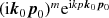 and
and  .
The angular integration can readily be carried out by using the
orthogonality relation of Legendre polynomials on the unit sphere, cf. (A3)
and (Landau & Lifshitz 1991)
.
The angular integration can readily be carried out by using the
orthogonality relation of Legendre polynomials on the unit sphere, cf. (A3)
and (Landau & Lifshitz 1991)
 (2.6)
(2.6)
In this way, we obtain the expansion of Dm, n in Legendre polynomials,
 (2.7)
(2.7)
These
distributions are real, and their symmetry properties with regard to a
simultaneous interchange of indices and arguments are evident from this
expansion. Dm, n
can be obtained from 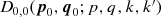 by multiple differentiation,
 (2.8)
(2.8)
We perform a radial integration of Dm, n, which defines the kernel
 (2.9)
(2.9)
This can also be written as, cf. (2.8),
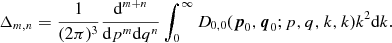 (2.10)
Employing the series expansion in equation (2.7), we obtain
 (2.11)
Here, the Bessel integral is a representation of the Dirac function (Jackson 1999)
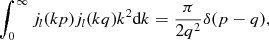 (2.12)
valid for integer l ≥ 0 and positive p and q. We use the Legendre representation of the delta function on the unit sphere, cf. (A2) and (A7),
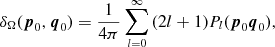 (2.13)
to factorize kernel (2.9),
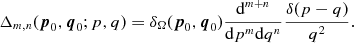 (2.14)
The delta function in Euclidean 3-space can be split as, cf. Appendix Appendix,
 (2.15)
so that
 (2.16)
This Cartesian representation of kernel (2.9) can directly be recovered from equations (2.5) and (2.10).
2.2 Temperature autocorrelation function
We define the correlation function of the Fourier components  in equation (2.1)
as
in equation (2.1)
as
 (2.17)
Isotropy requires the power spectrum g00(k)
to depend only on  , and the delta function reflects
homogeneity in Euclidean 3-space, so that the Fourier transform of
, and the delta function reflects
homogeneity in Euclidean 3-space, so that the Fourier transform of  only depends on the distance
  , cf. (2.21)
and (2.25).
, cf. (2.21)
and (2.25).
In polar coordinates, the Euclidean delta function factorizes as in equation (2.15), so that
 (2.18)
where  denotes the delta function on the
unit sphere, cf. Appendix Appendix
and equation (2.13).
Isotropy is ensured by
denotes the delta function on the
unit sphere, cf. Appendix Appendix
and equation (2.13).
Isotropy is ensured by  ,
which is the only angular dependent factor. We abandon homogeneity
(since the random field will ultimately be restricted to the unit
sphere) by replacing the singular radial factor g00(k)δ(k
− k′)/k2
by a more general kernel function,
,
which is the only angular dependent factor. We abandon homogeneity
(since the random field will ultimately be restricted to the unit
sphere) by replacing the singular radial factor g00(k)δ(k
− k′)/k2
by a more general kernel function,
 (2.19)
where k = k
k 0,  and
and
 (2.20)
Here, gmn(k) is an N-dimensional matrix, which will be chosen as positive-definite or semidefinite Hermitian. At this stage, we do not impose any symmetry requirements on gmn(k), which is thus an arbitrary complex N × N matrix. The homogeneous case (2.18) corresponds to N = 1.
The Fourier transform of the two-point function (2.19) is defined as
 (2.21)
where p = p
p 0 and
 . Zero subscripts denote unit
vectors. We may write this as
. Zero subscripts denote unit
vectors. We may write this as
 (2.22)
One of the angular integrations can readily be carried out by virtue of the delta function, cf. (2.5),
 (2.23)
We substitute Δ(k, k′) in equation (2.20), perform the partial integrations, use equation (2.8) and perform one integration by means of the delta function, to find the representation
 (2.24)
There are several ways to proceed. First, we may substitute
 (2.25)
Alternatively, we may use equation (2.8) to write (2.24) as
 (2.26)
Finally, we may substitute the Legendre expansion (2.7) of D0, 0 into equation (2.24) to find
 (2.27)
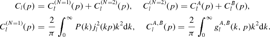
where we identified the multipole moments as
 (2.28)
One of the radial integrations in equation (2.28) is carried out by means of the delta function in Δ(k, k′), cf. (2.20), and we find, by multiple partial integration,
 (2.29)
This representation (equations (2.27), (2.28), (2.29)) of the Green function can be recovered by substituting the Legendre expansion (2.7) of Dm, n into (2.26).
We denote the two-point function (2.27)
by  , regarding it as an isotropic
kernel on the unit sphere depending on the angle
, regarding it as an isotropic
kernel on the unit sphere depending on the angle  and two arbitrary positive
scale-parameters p and p′,
cf. (2.19)
and (2.21).
The symmetry properties of
and two arbitrary positive
scale-parameters p and p′,
cf. (2.19)
and (2.21).
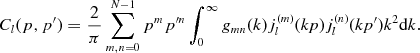
The symmetry properties of  with respect to p
and p′ depend on the coefficients Cl(p,
p′) in equation (2.29).
The Cl(p,
p′) are symmetric in p and p′
if the matrix gmn(k)
is symmetric, and they are real if gmn(k)
is real. If the matrix gmn(k)
is Hermitian, we find
with respect to p
and p′ depend on the coefficients Cl(p,
p′) in equation (2.29).
The Cl(p,
p′) are symmetric in p and p′
if the matrix gmn(k)
is symmetric, and they are real if gmn(k)
is real. If the matrix gmn(k)
is Hermitian, we find  . These symmetries of Cl(p,
p′) are inherited by the Green function
. These symmetries of Cl(p,
p′) are inherited by the Green function  .
.
If p′ = p (which
will be assumed in the sequel), we write Cl(p)
or simply Cl
for Cl(p,
p) in equation (2.29)
and  or
or  for the correlation function
  in equation (2.27).
The coefficients Cl(p)
are real if gmn(k)
is Hermitian or an arbitrary real matrix. Positivity of Cl(p)
is ensured if gmn(k)
is a positive-definite Hermitian (or real symmetric) matrix. The
condition Cl(p)
≥ 0 is satisfied if gmn(k)
is semidefinite. Thus,
in equation (2.27).
The coefficients Cl(p)
are real if gmn(k)
is Hermitian or an arbitrary real matrix. Positivity of Cl(p)
is ensured if gmn(k)
is a positive-definite Hermitian (or real symmetric) matrix. The
condition Cl(p)
≥ 0 is satisfied if gmn(k)
is semidefinite. Thus,  is a positive (semi)definite kernel
on the unit sphere if gmn(k)
is a positive (semi)definite Hermitian matrix. Reality, symmetry and
positive definiteness are the requirements for
is a positive (semi)definite kernel
on the unit sphere if gmn(k)
is a positive (semi)definite Hermitian matrix. Reality, symmetry and
positive definiteness are the requirements for  to be a Gaussian correlation
function, cf. Section 'OUTLOOK:
MULTICOMPONENT SPHERICAL RANDOM FIELDS'.
to be a Gaussian correlation
function, cf. Section 'OUTLOOK:
MULTICOMPONENT SPHERICAL RANDOM FIELDS'.
3 MULTIPOLE MOMENTS OF ISOTROPIC GAUSSIAN RANDOM FIELDS ON THE UNIT SPHERE
- Top of page
- ABSTRACT
- 1 INTRODUCTION
- 2 CMB TEMPERATURE FLUCTUATIONS: GENERAL SETTING
- 3 MULTIPOLE MOMENTS OF ISOTROPIC GAUSSIAN RANDOM FIELDS ON THE UNIT SPHERE
- 4 RECONSTRUCTION OF THE CMB TEMPERATURE POWER SPECTRUM
- 5 MULTIPOLE FINE STRUCTURE OF CMB TEMPERATURE FLUCTUATIONS
- 6 OUTLOOK: MULTICOMPONENT SPHERICAL RANDOM FIELDS
- 7 CONCLUSION
- REFERENCES
- Appendix A
- Appendix B
3.1 Hermitian spectral matrices defining angular power spectra
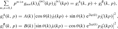
The Green function (2.27) is defined by multipole moments depending on a positive-definite or semidefinite Hermitian N × N matrix gmn(k), m, n = 0, … , N − 1, and a scale parameter p,
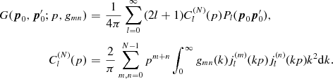 (3.1)
(3.1)
Multiple derivatives of the spherical Bessel functions jl(x)
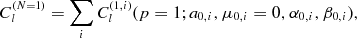
are indicated by superscripts (m) and (n).
We will also occasionally use a superscript (N)
for the matrix dimension, mainly N = 1 and 2 in
this paper. The case N = 1 can readily be
settled; we write P(k) for
density  to obtain the moments (3.1)
as
to obtain the moments (3.1)
as
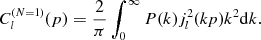 (3.2)
(3.2)
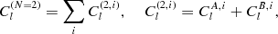
As for N = 2, we factorize the 2 × 2 matrix gmn(k) as
 (3.3)
(3.3)
where the diagonal matrix is defined by real constants A
≥ 0, B ≥ 0, and  is a unitary matrix of determinant
1, parametrized as
is a unitary matrix of determinant
1, parametrized as
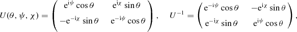 (3.4)
(3.4)
so that  . The Hermitian gmn(k)
thus reads
. The Hermitian gmn(k)
thus reads
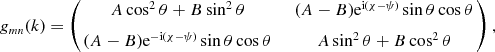 (3.5)
(3.5)
with m, n = 0, 1
and  . This parametrization covers all
two-dimensional positive semidefinite Hermitian matrices. gmn(k)
depends on four independent real parameters (A, B,
θ, ϕ), where ϕ = (χ − ψ)/2. These four parameters can be arbitrary real
functions of the spectral variable k. The case ϕ
= 0 is just a rotation in the Euclidean plane, resulting in a real
symmetric matrix. In higher dimensions, N ≥ 3, we
use subgroups Ui(θi,
ψi, χi)
as in equation (3.4)
to obtain an Euler-type parametrization of the Hermitian matrix, cf.
Appendix Appendix.
In the case that gmn(k)
factorizes as
. This parametrization covers all
two-dimensional positive semidefinite Hermitian matrices. gmn(k)
depends on four independent real parameters (A, B,
θ, ϕ), where ϕ = (χ − ψ)/2. These four parameters can be arbitrary real
functions of the spectral variable k. The case ϕ
= 0 is just a rotation in the Euclidean plane, resulting in a real
symmetric matrix. In higher dimensions, N ≥ 3, we
use subgroups Ui(θi,
ψi, χi)
as in equation (3.4)
to obtain an Euler-type parametrization of the Hermitian matrix, cf.
Appendix Appendix.
In the case that gmn(k)
factorizes as  , we can substitute in equation (3.1)
 (3.6)
(3.6)
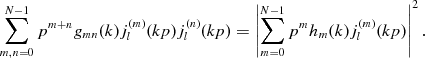
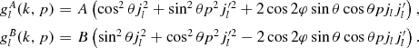
More generally, we can always split this quadratic form into a sum of N squares by diagonalization as in equation (3.3). In two dimensions, cf. (3.5),
 (3.7)
(3.7)
where we have put χ − ψ = 2ϕ. Here, the vectors hm(k)
defining the squares in equation (3.5)
are just the rows of matrix  in equation (3.4),
multiplied with a convenient phase factor and the root of the
respective coefficient in the diagonal matrix in equation (3.3);
the same holds for higher dimensions. A diagonal
in equation (3.4),
multiplied with a convenient phase factor and the root of the
respective coefficient in the diagonal matrix in equation (3.3);
the same holds for higher dimensions. A diagonal  results in a series of squared
derivatives
results in a series of squared
derivatives  . Positive definiteness of
  requires A
> 0 as well as B > 0.
requires A
> 0 as well as B > 0.
According to equation (3.7),
the multipole coefficients  in equation (3.1)
can be decomposed as
in equation (3.1)
can be decomposed as
 (3.8)
(3.8)
 (3.9)
(3.9)
where
 (3.10)
The argument of the Bessel functions is kp,
and the amplitudes and angles A, B,
θ and ϕ depend on the spectral variable k as
indicated in equation (3.7).
If we put 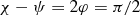 in matrix (3.5),
the mixed terms
in matrix (3.5),
the mixed terms  drop out.
When performing the integrations (3.9), it is convenient to write the spectral functions (3.10) linear in the harmonics,
 (3.11)
We note that  and
and  only differ by a change of sign of
the harmonics, apart from the amplitudes A and B,
and do not depend on the sign of the angle ϕ. The amplitudes A(k)
and B(k) as well as the
angles θ(k) and ϕ(k) will be
specified in equations (3.15)
and (3.16).
only differ by a change of sign of
the harmonics, apart from the amplitudes A and B,
and do not depend on the sign of the angle ϕ. The amplitudes A(k)
and B(k) as well as the
angles θ(k) and ϕ(k) will be
specified in equations (3.15)
and (3.16).
We consider linear combinations of the Green functions  in equation (3.1),
 (3.12)
where the summation is taken over a set of one- and
two-dimensional matrices gmn(k).
The multipole coefficients Cl(p)
in equation (3.12)
are obtained by adding the coefficients  of the respective components
  , cf. (3.1).
For instance, on adding
, cf. (3.1).
For instance, on adding  in equation (3.2)
and
in equation (3.2)
and  in equations (3.8)
and (3.9),
we find
in equations (3.8)
and (3.9),
we find
 (3.13)
As for the integral kernels, P(k)
is a density specified in equation (3.14),
and the spectral functions  and
and  are stated in equation (3.11),
with angular parametrization (3.15)
and amplitudes (3.16).
More generally, any Green function (3.12) obtained by summation over a
finite set of positive (semi)definite Hermitian matrices
are stated in equation (3.11),
with angular parametrization (3.15)
and amplitudes (3.16).
More generally, any Green function (3.12) obtained by summation over a
finite set of positive (semi)definite Hermitian matrices  (of the same or varying dimension N)
is a positive-definite or semidefinite Hermitian kernel, and the same
holds for linear combinations with positive coefficients. We may also
use different scale parameters p in each of the
component functions
(of the same or varying dimension N)
is a positive-definite or semidefinite Hermitian kernel, and the same
holds for linear combinations with positive coefficients. We may also
use different scale parameters p in each of the
component functions  in equation (3.12).
In the following, we will perform a summation over one- and
two-dimensional matrices as in equation (3.13),
using the same scale parameter p in each
component
in equation (3.12).
In the following, we will perform a summation over one- and
two-dimensional matrices as in equation (3.13),
using the same scale parameter p in each
component  .
.
3.2 Spectral parametrization of multipole moments: Gaussian power-law densities and Kummer distributions
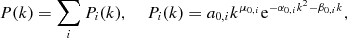
As for the coefficients  in equation (3.2),
we parametrize the kernel P(k)
with a series of Gaussian power-law densities,
in equation (3.2),
we parametrize the kernel P(k)
with a series of Gaussian power-law densities,
 (3.14)
with amplitudes a0, i > 0 and real exponents μ0, i, β0, i, and α0, i > 0. This series corresponds to a summation over a set of one-dimensional matrices in equation (3.12).
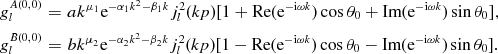
Regarding the coefficients  in equation (3.8),
we need to specify the k dependence of the angles
and amplitudes in the 2 × 2 matrix (3.5)
and the associated spectral functions
in equation (3.8),
we need to specify the k dependence of the angles
and amplitudes in the 2 × 2 matrix (3.5)
and the associated spectral functions  in (3.11).
We use a linear k parametrization of the angles,
in (3.11).
We use a linear k parametrization of the angles,
 (3.15)
where ω, θ0, ω0 and ϕ0 are real constants. When performing the CMB temperature fit, it suffices to put θ0 = 0 and ϕ(k) = 0 from the outset. The amplitudes are Gaussian power laws like in equation (3.14),
 (3.16)
with a ≥ 0, b ≥ 0
and real exponents μ1, 2, β1, 2
and α1, 2. In the CMB temperature fit, we use α1,
2 = 0 and β1, 2 > 0, that is,
power-law densities with exponential cut-off. If the amplitudes a
and b in equation (3.16)
have opposite sign, the Hermitian spectral matrix (3.5)
is indefinite, but the multipole coefficients  in equation (3.13)
can still be positive for all l. Similarly, if
some of the Gaussian amplitudes a0, i
in equation (3.14)
are negative, the total moments Cl(p)
in equation (3.13)
can still be positive. Positivity of the amplitudes is sufficient but
not necessary to ensure a positive-definite kernel (3.12).
in equation (3.13)
can still be positive for all l. Similarly, if
some of the Gaussian amplitudes a0, i
in equation (3.14)
are negative, the total moments Cl(p)
in equation (3.13)
can still be positive. Positivity of the amplitudes is sufficient but
not necessary to ensure a positive-definite kernel (3.12).
On substituting the angles (3.15)
and amplitudes (3.16)
into the spectral functions  in equation (3.11),
we find
in equation (3.11),
we find
 (3.17)
where  and
and  denote the terms depending on
  in equation (3.11),
 (3.18)
The terms  and
and  in equation (3.17)
contain the squared derivatives
in equation (3.17)
contain the squared derivatives  as factor,
 (3.19)
The contributions  and
and  to the spectral functions (3.17)
stem from the mixed terms
to the spectral functions (3.17)
stem from the mixed terms  in equation (3.11),
 (3.20)
and
 (3.21)
The multipole coefficients  in equation (3.13)
are obtained by integration of the spectral functions (3.17),
(3.18), (3.19), (3.20), (3.21), cf. Section 'RECONSTRUCTION
OF THE CMB TEMPERATURE POWER SPECTRUM'. We have written the
harmonics depending on the spectral variable k as
real and imaginary parts of exponentials to facilitate this integration.
in equation (3.13)
are obtained by integration of the spectral functions (3.17),
(3.18), (3.19), (3.20), (3.21), cf. Section 'RECONSTRUCTION
OF THE CMB TEMPERATURE POWER SPECTRUM'. We have written the
harmonics depending on the spectral variable k as
real and imaginary parts of exponentials to facilitate this integration.
4 RECONSTRUCTION OF THE CMB TEMPERATURE POWER SPECTRUM
- Top of page
- ABSTRACT
- 1 INTRODUCTION
- 2 CMB TEMPERATURE FLUCTUATIONS: GENERAL SETTING
- 3 MULTIPOLE MOMENTS OF ISOTROPIC GAUSSIAN RANDOM FIELDS ON THE UNIT SPHERE
- 4 RECONSTRUCTION OF THE CMB TEMPERATURE POWER SPECTRUM
- 5 MULTIPOLE FINE STRUCTURE OF CMB TEMPERATURE FLUCTUATIONS
- 6 OUTLOOK: MULTICOMPONENT SPHERICAL RANDOM FIELDS
- 7 CONCLUSION
- REFERENCES
- Appendix A
- Appendix B
4.1 Assembling the multipole coefficients: integrated spectral functions
We start with the Bessel integral
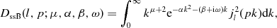 (4.1)
(4.1)
with real exponents α ≥ 0, β, ω and μ. If α = 0, we assume a
positive exponent β. The multipole component  in equation (3.13),
generated by density P(k) in
equation (3.14),
reads
in equation (3.13),
generated by density P(k) in
equation (3.14),
reads
 (4.2)
(4.2)
Occasionally, we will indicate the parameter dependence, 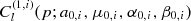 . In the figures, we label the
contribution of the components
. In the figures, we label the
contribution of the components  to the total multipole coefficients
Cl by Pi.
The low-l
region of the CMB temperature power spectrum, the main peak, as well as
the crossover to the modulated decaying slope is an additive
combination of eight Gaussian peaks, cf. Figs 1
and 2, so
that the summation index in equation (4.2)
runs from i = 1 to 8, cf. Table 1.
A detailed description of the multipole fit in the Gaussian regime, in
particular of the fitting parameters of the Gaussian peaks recorded in
Table 1, is
given in Section 'Gaussian
multipole moments in the low-l region',
after having discussed the scaling relations and the scale-invariant
limit of the Gaussian and oscillatory multipole components in Section 'Scaling
relations for the multipole moments'.
to the total multipole coefficients
Cl by Pi.
The low-l
region of the CMB temperature power spectrum, the main peak, as well as
the crossover to the modulated decaying slope is an additive
combination of eight Gaussian peaks, cf. Figs 1
and 2, so
that the summation index in equation (4.2)
runs from i = 1 to 8, cf. Table 1.
A detailed description of the multipole fit in the Gaussian regime, in
particular of the fitting parameters of the Gaussian peaks recorded in
Table 1, is
given in Section 'Gaussian
multipole moments in the low-l region',
after having discussed the scaling relations and the scale-invariant
limit of the Gaussian and oscillatory multipole components in Section 'Scaling
relations for the multipole moments'.
| i | a0, i | α0, i | β0, i | r0, i = −α0, i/β0, i |
|---|---|---|---|---|
| 1 | 2.5 × 10² | 6.25 × 10⁻² | −0.25 | 0.25 |
| 2 | 1.5 | 1.47 × 10⁻² | −0.3 | 4.9 × 10⁻² |
| 3 | 5.0 × 10⁻⁵ | 7.0 × 10⁻³ | −0.5 | 1.4 × 10⁻² |
| 4 | 2.1 × 10⁻² | 6.6 × 10⁻⁴ | −0.06 | 1.1 × 10⁻² |
| 5 | 3.6 × 10⁻⁵ | 4.5 × 10⁻⁴ | −0.1 | 4.5 × 10⁻³ |
| 6 | 3.05 × 10⁻³ | 6.26 × 10⁻⁵ | −0.02 | 3.13 × 10⁻³ |
| 7 | 1.0 × 10⁻¹⁶ | 1.067 × 10⁻⁴ | −0.11 | 9.7 × 10⁻⁴ |
| 8 | 9.5 × 10⁻¹⁹ | 5.04 × 10⁻⁵ | −0.08 | 6.3 × 10⁻⁴ |
 , cf.
, cf.  are obtained by averaging squared
spherical Bessel functions with Gaussian densities
are obtained by averaging squared
spherical Bessel functions with Gaussian densities  , cf.
, cf. As for the oscillatory multipole component  in equation (3.13),
generated by the Hermitian kernel (3.5),
we replace the squared spherical Bessel function in integral (4.1)
by a product of derivatives,
in equation (3.13),
generated by the Hermitian kernel (3.5),
we replace the squared spherical Bessel function in integral (4.1)
by a product of derivatives,
 (4.3)
(4.3)
so that  . These integrals are convergent for
μ > −3 and
. These integrals are convergent for
μ > −3 and  or
or  and β > 0. The coefficients
  can be split, according to
equations (3.13)
and (3.17),
(3.18), (3.19), (3.20), (3.21), as
can be split, according to
equations (3.13)
and (3.17),
(3.18), (3.19), (3.20), (3.21), as
 (4.4)
(4.4)
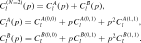
The superscript (0,0) indicates the  -dependent multipole component
(stemming from the spectral functions
-dependent multipole component
(stemming from the spectral functions  and
and  in equation (3.18)),
calculated as linear combination of the averages
in equation (3.18)),
calculated as linear combination of the averages  in equation (4.3):
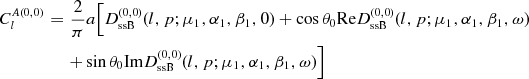 (4.5)
(4.5)
and
 (4.6)
(4.6)
The parameter dependence of these moments is  and
and  . The frequency ω and the angle θ0
stem from the parametrization (3.15)
of the matrix kernel (3.5).
We also note that μ1, 2 > −3 is a
requirement for the coefficients
. The frequency ω and the angle θ0
stem from the parametrization (3.15)
of the matrix kernel (3.5).
We also note that μ1, 2 > −3 is a
requirement for the coefficients  and
and  to be convergent, and similarly for
 in equation (4.2),
where μ0, i > −3 is
required. The zeroth multipole moment Cl=
0 of the CMB temperature fit depicted in the figures is
safely finite (and positive), but does not show due to the l(l
+ 1) normalization of the moments. A preferable though less customary
normalization of the Cl
plots is (l + 1/2)2.
in equation (4.2),
where μ0, i > −3 is
required. The zeroth multipole moment Cl=
0 of the CMB temperature fit depicted in the figures is
safely finite (and positive), but does not show due to the l(l
+ 1) normalization of the moments. A preferable though less customary
normalization of the Cl
plots is (l + 1/2)2.
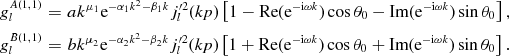
The superscript (1,1) in equation (4.4)
indicates the  -dependent contribution to the
multipole moments, defined by
-dependent contribution to the
multipole moments, defined by  and
and  in equation (3.19),
and calculated by means of the integrals
in equation (3.19),
and calculated by means of the integrals  in equation (4.3):
 (4.7)
(4.7)
and
 (4.8)
(4.8)
The parameter dependence is the same as of  and
and  , cf. the text after equation (4.6).
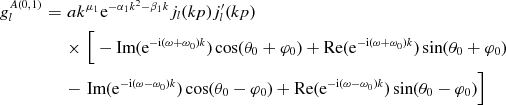
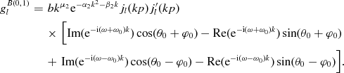
The superscript (0,1) in equation (4.4)
labels the multipole contribution of the mixed coefficients  , stemming from
  in equation (3.20)
and
in equation (3.20)
and  in equation (3.21).
We find, by means of the integrals
in equation (3.21).
We find, by means of the integrals  in equation (4.3),
 (4.9)
(4.9)
and
 (4.10)
The angles θ0 and ϕ0
and the frequencies ω and ω0 are arbitrary
constants, fitting parameters in the angular parametrization (3.15)
of the matrix kernel. If we put ω0 = 0 and  , the coefficients
  and
and  vanish, cf. the text after equation
(3.10).
Otherwise, their parameter dependence is
vanish, cf. the text after equation
(3.10).
Otherwise, their parameter dependence is  and
and  , and the same holds for the total
coefficients
, and the same holds for the total
coefficients  and
and  in equation (4.4).
As in equation (4.2),
we may perform a summation over a set of 2 × 2 matrices, cf. (3.12),
in equation (4.4).
As in equation (4.2),
we may perform a summation over a set of 2 × 2 matrices, cf. (3.12),
 (4.11)
The index i labels the parameter sets
defining the two-dimensional matrices, cf. (3.5),
(3.15)
and (3.16),
and each component function is compiled as stated in equations (4.4),
(4.5), (4.6), (4.7), (4.8), (4.9), (4.10). In the CMB
temperature fit, we put θ0, i
= ω0, i = ϕ0, i
= 0 as well as α1, i = α2,
i = 0 from the outset, so that the
Bessel derivatives in equation (4.3)
are averaged with a power-law density with modulated exponential
cut-off (Kummer distribution). In the figures, we use the shortcut  to label the multipole component
  and
and  for
for  , as well as
  for their sum
  , cf. the dotted curves in Figs 3
and 4.
The fit of the CMB power spectrum is performed with two two-dimensional
matrices, which suffice to adequately reproduce the oscillatory and
high-l regimes, so that the summation in equation (4.11)
is over i = 1, 2, cf. Table 2.
The multipole fit in these regimes and the fitting parameters in Table 2
are explained in Section 'Oscillatory
multipole spectrum generated by Kummer distributions in the
transitional and high-l regimes'.
, cf. the dotted curves in Figs 3
and 4.
The fit of the CMB power spectrum is performed with two two-dimensional
matrices, which suffice to adequately reproduce the oscillatory and
high-l regimes, so that the summation in equation (4.11)
is over i = 1, 2, cf. Table 2.
The multipole fit in these regimes and the fitting parameters in Table 2
are explained in Section 'Oscillatory
multipole spectrum generated by Kummer distributions in the
transitional and high-l regimes'.
| i | ai | μ1, i | β1, i | bi | μ2, i | β2, i | ωi |
|---|---|---|---|---|---|---|---|
| 1 | 2.6 × 10⁻⁶ | 1 | 4.6 × 10⁻³ | 5.4 × 10⁻⁵ | 0 | 2.3 × 10⁻³ | 2.15 × 10⁻² |
| 2 | 6.6 × 10⁻¹³ | 1 | 2.1 × 10⁻⁴ | 0 | – | – | 0 |
 ,
,  and
and  , i = 1, 2, in
Figs
, i = 1, 2, in
Figs  stands for the oscillatory
multipole component
stands for the oscillatory
multipole component  ,
,  for
for  and
and  for
for  , cf.
, cf.  and
and  moments are linear combinations of
squared spherical Bessel functions averaged with Kummer distributions
moments are linear combinations of
squared spherical Bessel functions averaged with Kummer distributions  (power laws with modulated
exponential cut-off), cf. Section
(power laws with modulated
exponential cut-off), cf. Section  and
and  are listed in the first row, and of
 in the second
The total multipole coefficients Cl are obtained by adding the contribution of the one- and two-dimensional matrix kernels in equations (4.2) and (4.11),
 (4.12)
The component  is a Gaussian average which
dominates the low-l regime including the main
peak, cf. the text after equation (4.2).
The oscillatory component
is a Gaussian average which
dominates the low-l regime including the main
peak, cf. the text after equation (4.2).
The oscillatory component  generated by Kummer distributions reproduces the decaying modulated
slope and the subsequent power-law ascent with exponential cut-off, cf.
Figs 4 and 5.
The crossover between the Gaussian main peak and the modulated slope
consists of two secondary peaks of nearly equal height, to which the
Gaussian and oscillatory multipole components in equation (4.12)
contribute in equal measure, cf. Figs 9-11.
generated by Kummer distributions reproduces the decaying modulated
slope and the subsequent power-law ascent with exponential cut-off, cf.
Figs 4 and 5.
The crossover between the Gaussian main peak and the modulated slope
consists of two secondary peaks of nearly equal height, to which the
Gaussian and oscillatory multipole components in equation (4.12)
contribute in equal measure, cf. Figs 9-11.
4.2 Scaling relations for the multipole moments
The Bessel integrals in equations (4.1) and (4.3) satisfy the scaling relation
 (4.13)
Applying this to the Gaussian multipole components  in equation (4.2),
we find
in equation (4.2),
we find
 (4.14)
where the parameter p has been scaled into the arguments
 (4.15)
In particular, the scale factor p−μ
− 3 in equation (4.13)
is absorbed by the indicated rescaling of the amplitude a0,
i of the  , cf. (4.2).
Thus, the p dependence of the Gaussian
coefficients
, cf. (4.2).
Thus, the p dependence of the Gaussian
coefficients  can be completely absorbed in the
fitting parameters, resulting in scale invariance. In effect, we can
put p = 1 and use
can be completely absorbed in the
fitting parameters, resulting in scale invariance. In effect, we can
put p = 1 and use  in the CMB temperature fit, with
the indicated variables as independent fitting parameters, cf. Table 1.
in the CMB temperature fit, with
the indicated variables as independent fitting parameters, cf. Table 1.
We turn to the p scaling of the
oscillatory multipole moments in equations (4.4)
and (4.11),
generated by the Hermitian kernel (3.5). The component functions  and
and  in equations (4.5)
and (4.6)
are scale invariant,
in equations (4.5)
and (4.6)
are scale invariant,
 (4.16)
as we can absorb the scaling parameter p in the fitting parameters,
 (4.17)
The coefficients  and
and  in equations (4.7)
and (4.8)
scale like
in equations (4.7)
and (4.8)
scale like  and
and  in equation (4.16).
The mixed components
in equation (4.16).
The mixed components  and
and  in equations (4.9)
and (4.10)
are likewise scale invariant,
in equations (4.9)
and (4.10)
are likewise scale invariant,
 (4.18)
with the rescaled parameters listed in equation (4.17)
and  .
.
Thus, the coefficients  and
and  in equations (4.4)
and (4.11)
reduce to second-order polynomials in p if we use
the rescaled parameters (4.17)
and
in equations (4.4)
and (4.11)
reduce to second-order polynomials in p if we use
the rescaled parameters (4.17)
and  as independent fitting parameters:
 (4.19)
and
 (4.20)
In the Gaussian multipole components (4.14),
the scale parameter p can be absorbed in the
fitting parameters, as done in equation (4.15).
In contrast, in the oscillatory components  compiled in equations (4.11),
(4.19)
and (4.20),
there remains an explicit p dependence breaking
the scale invariance. The scale parameter p
enters as an additional fitting parameter, as a weight factor
determining the contribution of the Bessel products
compiled in equations (4.11),
(4.19)
and (4.20),
there remains an explicit p dependence breaking
the scale invariance. The scale parameter p
enters as an additional fitting parameter, as a weight factor
determining the contribution of the Bessel products  ,
,  and
and  (weighted by 1, p
and p2, respectively) to
the multipole moments. There is no other p
dependence, as the rescaled variables indicated by a tilde in equations
(4.19)
and (4.20)
are independent fitting parameters. Scale invariance is attained in the
limit p → 0, where the coefficients
(weighted by 1, p
and p2, respectively) to
the multipole moments. There is no other p
dependence, as the rescaled variables indicated by a tilde in equations
(4.19)
and (4.20)
are independent fitting parameters. Scale invariance is attained in the
limit p → 0, where the coefficients  and
and  coincide with
  and
and  , respectively. In effect, this
means to discard the linear and quadratic p terms
in equation (4.4)
(which give the multipole contributions of the
, respectively. In effect, this
means to discard the linear and quadratic p terms
in equation (4.4)
(which give the multipole contributions of the  and
and  products), and to put p
= 1 in the explicit expressions for
products), and to put p
= 1 in the explicit expressions for  and
and  in equations (4.5)
and (4.6).
The rescaled variables in
in equations (4.5)
and (4.6).
The rescaled variables in  and
and  can be renamed to the original
ones, cf. (4.17),
to arrive at
can be renamed to the original
ones, cf. (4.17),
to arrive at
 (4.21)
The multipole components (4.19) and (4.20) thus reduce to (4.21) in the scale-invariant limit p = 0 adopted in the CMB temperature power fit. The fitting parameters indicated as arguments in (4.21) are listed in Table 2.
5 MULTIPOLE FINE STRUCTURE OF CMB TEMPERATURE FLUCTUATIONS
- Top of page
- ABSTRACT
- 1 INTRODUCTION
- 2 CMB TEMPERATURE FLUCTUATIONS: GENERAL SETTING
- 3 MULTIPOLE MOMENTS OF ISOTROPIC GAUSSIAN RANDOM FIELDS ON THE UNIT SPHERE
- 4 RECONSTRUCTION OF THE CMB TEMPERATURE POWER SPECTRUM
- 5 MULTIPOLE FINE STRUCTURE OF CMB TEMPERATURE FLUCTUATIONS
- 6 OUTLOOK: MULTICOMPONENT SPHERICAL RANDOM FIELDS
- 7 CONCLUSION
- REFERENCES
- Appendix A
- Appendix B
5.1 Gaussian multipole moments in the low-l region
To summarize, the CMB temperature multipole moments,
 (5.1)
(5.1)
plotted in Figs 1-13, are assembled from Gaussian and oscillatory components. The Gaussian moments, cf. (4.14),
 (5.2)
(5.2)
consist of Gaussian averages  defined by the Bessel integrals in
equations (4.1)
and (4.2).
In the figures, the plots of the individual components
defined by the Bessel integrals in
equations (4.1)
and (4.2).
In the figures, the plots of the individual components  , i = 1, … ,
8, are labelled by Pi,
which stands for the Gaussian density (3.14)
generating the respective coefficients
, i = 1, … ,
8, are labelled by Pi,
which stands for the Gaussian density (3.14)
generating the respective coefficients  . In equation (5.2),
the power-law exponents μ0, i
have been put to zero from the outset; the remaining fitting parameters
α0, i, β0, i
and a0, i
determining the location, width and amplitude of the peaks Pi
= 1, … , 8 are listed in Table 1.
. In equation (5.2),
the power-law exponents μ0, i
have been put to zero from the outset; the remaining fitting parameters
α0, i, β0, i
and a0, i
determining the location, width and amplitude of the peaks Pi
= 1, … , 8 are listed in Table 1.
The peaks labelled Pi
in the figures (dashed curves) are the l plots of
the Gaussian multipole components  , cf. (4.2),
where DssB is the Bessel
integral (4.1).
As a rule of thumb, the ratio r0, i
= −α0, i/β0, i
listed in Table 1
determines the location of the peak Pi;
a smaller r0, i
shifts the peak to the right, towards higher l
values. The negative exponent β0, i
determines the width of the peak, a smaller |β0, i|
resulting in a larger width. These qualitative features of the averages
(4.1)
hold particularly well for peaks at moderate and high l,
such as P7 and P8
in the first transitional regime, cf. Fig. 10;
the high-l asymptotics of the Bessel integrals in
equations (4.1)
and (4.3)
and their numerical evaluation will be discussed elsewhere. The
Gaussian component (5.2)
dominates the CMB temperature fit at low l, up to
about l ∼ 100, cf. Figs 6
and 7. In
this regime, the fit Cl
is obtained by adding the Gaussian peaks Pi
and a tiny admixture of the oscillatory component
, cf. (4.2),
where DssB is the Bessel
integral (4.1).
As a rule of thumb, the ratio r0, i
= −α0, i/β0, i
listed in Table 1
determines the location of the peak Pi;
a smaller r0, i
shifts the peak to the right, towards higher l
values. The negative exponent β0, i
determines the width of the peak, a smaller |β0, i|
resulting in a larger width. These qualitative features of the averages
(4.1)
hold particularly well for peaks at moderate and high l,
such as P7 and P8
in the first transitional regime, cf. Fig. 10;
the high-l asymptotics of the Bessel integrals in
equations (4.1)
and (4.3)
and their numerical evaluation will be discussed elsewhere. The
Gaussian component (5.2)
dominates the CMB temperature fit at low l, up to
about l ∼ 100, cf. Figs 6
and 7. In
this regime, the fit Cl
is obtained by adding the Gaussian peaks Pi
and a tiny admixture of the oscillatory component  in equation (5.1),
emerging at the lower edge of Fig. 6 as
dotted curve
in equation (5.1),
emerging at the lower edge of Fig. 6 as
dotted curve  . The main peak shown in Figs 8
and 9 is
essentially generated by the Gaussian peak P6,
with admixtures of smaller adjacent Gaussian peaks and the mentioned
oscillatory component
. The main peak shown in Figs 8
and 9 is
essentially generated by the Gaussian peak P6,
with admixtures of smaller adjacent Gaussian peaks and the mentioned
oscillatory component  (discussed in Section 'Oscillatory
multipole spectrum generated by Kummer distributions in the
transitional and high-l regimes'), which
becomes more dominant with increasing l. The main
peak covers the multipole region 100 ≤ l ≤ 400.
(discussed in Section 'Oscillatory
multipole spectrum generated by Kummer distributions in the
transitional and high-l regimes'), which
becomes more dominant with increasing l. The main
peak covers the multipole region 100 ≤ l ≤ 400.
5.2 Oscillatory multipole spectrum generated by Kummer distributions in the transitional and high-l regimes
The oscillatory moments  in equation (5.1)
are compiled as, cf. (4.11)
and (4.21),
in equation (5.1)
are compiled as, cf. (4.11)
and (4.21),
 (5.3)
(5.3)
where we use the shortcuts
 (5.4)
(5.4)
for the component functions  and
and  , which are explicitly stated in
equations (4.5)
and (4.6)
as linear combinations of the Bessel averages (4.3).
In equation (5.4),
we have put the exponents α1, i
and α2, i to zero from the
outset, which means to drop the quadratic term in the exponentials in
equation (4.3).
We have also equated the angle θ0, i
to zero, which appears in the angular parametrization (3.15)
of the Hermitian spectral matrices generating the oscillatory moments.
The CMB temperature fit in Figs 1-13
is performed with the total moments Cl
in equation (5.1),
obtained by adding the Gaussian moments (5.2)
specified in Table 1 to the
oscillatory moments listed in equations (5.3)
and (5.4)
and Table 2.
, which are explicitly stated in
equations (4.5)
and (4.6)
as linear combinations of the Bessel averages (4.3).
In equation (5.4),
we have put the exponents α1, i
and α2, i to zero from the
outset, which means to drop the quadratic term in the exponentials in
equation (4.3).
We have also equated the angle θ0, i
to zero, which appears in the angular parametrization (3.15)
of the Hermitian spectral matrices generating the oscillatory moments.
The CMB temperature fit in Figs 1-13
is performed with the total moments Cl
in equation (5.1),
obtained by adding the Gaussian moments (5.2)
specified in Table 1 to the
oscillatory moments listed in equations (5.3)
and (5.4)
and Table 2.
The decaying modulated slope in Figs 11
and 12 and
the subsequent power-law rise of Cl
in Fig. 13 are
generated by the multipole component (5.3);
the Gaussian peaks (5.2)
do not affect multipoles beyond l ∼ 1000. The
plots of the individual components  in equation (5.4)
are labelled by
in equation (5.4)
are labelled by  in the figures, the plot of
  by
by  and the plot of the sum
  in equation (5.3)
by
in equation (5.3)
by  . The component
  (labelled
  suffices to model the high-l
regime, so that we have put
suffices to model the high-l
regime, so that we have put  .
.  ,
,  and
and  stand for Kummer distributions
  in the Bessel averages (4.3)
defining the moments
in the Bessel averages (4.3)
defining the moments  ,
,  and
and  in equation (5.4),
cf. Table 2.
in equation (5.4),
cf. Table 2.
In the first row of Table 2, we
have listed the fitting parameters of the moments  and
and  , which constitute the oscillatory
multipole component generating the decaying intermediate-l
slope in Figs 11 and 12.
In the interval 1000 ≤ l ≤ 2500, the multipole
fit essentially consists of these two components,
, which constitute the oscillatory
multipole component generating the decaying intermediate-l
slope in Figs 11 and 12.
In the interval 1000 ≤ l ≤ 2500, the multipole
fit essentially consists of these two components,  , whose plots (dotted curves) are
labelled
, whose plots (dotted curves) are
labelled  and
and  in the figures. The moments Cl
are obtained by adding these two curves, cf. Figs 11
and 12; the
contributions of the Gaussian peak P8
and of the ascending slope
in the figures. The moments Cl
are obtained by adding these two curves, cf. Figs 11
and 12; the
contributions of the Gaussian peak P8
and of the ascending slope  (both indicated at the lower edge
of Fig. 12) are
negligible in this interval. The second row of Table 2
contains the fitting parameters of the moments
(both indicated at the lower edge
of Fig. 12) are
negligible in this interval. The second row of Table 2
contains the fitting parameters of the moments  (depicted as dotted curve
  in Figs 12
and 13),
which dominate the fit above l ∼ 4000,
in Figs 12
and 13),
which dominate the fit above l ∼ 4000,  . This component generates the
extended non-Gaussian peak at l ≈ 15 400 in Fig. 5.
. This component generates the
extended non-Gaussian peak at l ≈ 15 400 in Fig. 5.
In Section 'Gaussian
multipole moments in the low-l region',
we have studied the Gaussian regime 0 ≤ l ≤ 400,
cf. Figs 6-9.
In this section, we discuss the intermediate oscillatory regime, the
interval 1000 ≤ l ≤ 2500 containing the modulated
decaying slope of Cl,
cf. Figs 11 and 12,
as well as the high-l regime above l
∼ 4000, cf. Fig. 13.
There are two transitional regimes. The first, 400 ≤ l
≤ 1000, is the crossover region from the Gaussian to the oscillatory
regime depicted in Figs 8-11.
The crossover consists of two secondary peaks of nearly the same height
following the main peak. These peaks are the result of pronounced
modulations in the oscillatory component (comprising the moments  and
and  discussed above and depicted as
dotted curves
discussed above and depicted as
dotted curves  and
and  and of two Gaussian peaks P7
and P8 located in this
transitional region. The fit in the crossover interval 400 ≤ l
≤ 1000 is thus obtained as
and of two Gaussian peaks P7
and P8 located in this
transitional region. The fit in the crossover interval 400 ≤ l
≤ 1000 is thus obtained as  , with a small admixture from the
main peak P6, cf. Fig. 10.
The second transitional regime is the interval 2500 ≤ l
≤ 4000, cf. Fig. 12,
joining the oscillatory multipole component
, with a small admixture from the
main peak P6, cf. Fig. 10.
The second transitional regime is the interval 2500 ≤ l
≤ 4000, cf. Fig. 12,
joining the oscillatory multipole component  to the ascending power-law slope of
the high-l component
to the ascending power-law slope of
the high-l component  . The fit
  in this crossover region is
obtained by adding the exponentially damped tail
in this crossover region is
obtained by adding the exponentially damped tail  to the emerging rising slope
  , cf. Figs 12
and 13, the
latter dominating the multipole spectrum above l
∼ 4000.
, cf. Figs 12
and 13, the
latter dominating the multipole spectrum above l
∼ 4000.
6 OUTLOOK: MULTICOMPONENT SPHERICAL RANDOM FIELDS
- Top of page
- ABSTRACT
- 1 INTRODUCTION
- 2 CMB TEMPERATURE FLUCTUATIONS: GENERAL SETTING
- 3 MULTIPOLE MOMENTS OF ISOTROPIC GAUSSIAN RANDOM FIELDS ON THE UNIT SPHERE
- 4 RECONSTRUCTION OF THE CMB TEMPERATURE POWER SPECTRUM
- 5 MULTIPOLE FINE STRUCTURE OF CMB TEMPERATURE FLUCTUATIONS
- 6 OUTLOOK: MULTICOMPONENT SPHERICAL RANDOM FIELDS
- 7 CONCLUSION
- REFERENCES
- Appendix A
- Appendix B
We consider T(p)
as a component of a multicomponent scalar field  on the sphere, where the index i
= T, E, B,
… labels, for instance, temperature, E and B
polarization, circular polarization if detectable, an angular galaxy
distribution, etc. The temperature field T(p)
reads in this notation
on the sphere, where the index i
= T, E, B,
… labels, for instance, temperature, E and B
polarization, circular polarization if detectable, an angular galaxy
distribution, etc. The temperature field T(p)
reads in this notation  . The counterpart to the Green
function
. The counterpart to the Green
function  in equation (2.27)
is
in equation (2.27)
is
 (6.1)
(6.1)
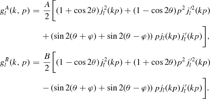
The multipole coefficients Cij;
l are symmetric in i
and j,
assembled by averaging squared spherical Bessel functions with Gaussian
power laws and Kummer distributions as explained in Sections 'MULTIPOLE
MOMENTS OF ISOTROPIC GAUSSIAN RANDOM FIELDS ON THE UNIT SPHERE'
and 'RECONSTRUCTION
OF THE CMB TEMPERATURE POWER SPECTRUM'.
The Hermitian spectral kernels defining the off-diagonal elements need
not be positive definite, so that the diagonal matrices in the
decomposition (3.3)
and (B1)
can have negative coefficients, also see the text after equation (3.16).
The inverse  is defined by the same series with
the real symmetric multipole coefficients Cij;
l replaced by the inverse matrices
is defined by the same series with
the real symmetric multipole coefficients Cij;
l replaced by the inverse matrices  . By making use of the orthogonality
relation (2.6)
of Legendre polynomials and the series representation (2.13) of the
delta function on the unit sphere, we find
. By making use of the orthogonality
relation (2.6)
of Legendre polynomials and the series representation (2.13) of the
delta function on the unit sphere, we find
 (6.2)
(6.2)
The kernels  are real and symmetric, depending
only on
are real and symmetric, depending
only on  and the scale parameter p.
Due to the assumed isotropy, it suffices to expand the Green function
in Legendre polynomials rather than in products of spherical harmonics.
Isotropy is crucial if the CMB rest frame is to define an absolute
frame of reference (Tomaschitz 2012).
and the scale parameter p.
Due to the assumed isotropy, it suffices to expand the Green function
in Legendre polynomials rather than in products of spherical harmonics.
Isotropy is crucial if the CMB rest frame is to define an absolute
frame of reference (Tomaschitz 2012).
The matrices Cij;
l(p) can be
regarded as positive definite, as the positive CTT;
l(p) component
usually overpowers all others, so that the inverse correlation function
(6.1)
is a Gaussian kernel. [Even if the Cij;
l are not invertible, one can try the
characteristic functional (6.6)
as a starting point, instead of the Gaussian density (6.5),
to generate n-point
correlations.] As we will only use unit vectors in this section, we
drop the zero subscripts as well as the scale parameter as argument,
writing  or
or  for the Green function (6.1)
and its inverse on the unit sphere
for the Green function (6.1)
and its inverse on the unit sphere  . Spherical integrations are denoted
by the solid-angle element
. Spherical integrations are denoted
by the solid-angle element  , and the real random variables by
  . The multipole expansion (6.1)
can be inverted by way of the orthogonality relation (2.6)
and Pl(1)
= 1,
. The multipole expansion (6.1)
can be inverted by way of the orthogonality relation (2.6)
and Pl(1)
= 1,
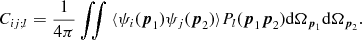 (6.3)
(6.3)
The second solid-angle integration has been added for symmetry reasons.
The observationally determined Green function is found by
specifying the multipole coefficients in equations (6.1)
and (6.3)
as  , where
  are coefficients extracted from the
two-dimensional CMB maps, by replacing the average
are coefficients extracted from the
two-dimensional CMB maps, by replacing the average  in equation (6.3)
by the product
in equation (6.3)
by the product  of the measured field components.
We may substitute the integral representation of the coefficients
of the measured field components.
We may substitute the integral representation of the coefficients  (i.e. equation (6.3)
without angle brackets) into the Legendre series (6.1),
interchange integration and summation, and use the completeness
relation (A4)
of the Legendre polynomials. In this way, we arrive at an integral
representation of the Green function equivalent to the Legendre series (6.1)
(with
(i.e. equation (6.3)
without angle brackets) into the Legendre series (6.1),
interchange integration and summation, and use the completeness
relation (A4)
of the Legendre polynomials. In this way, we arrive at an integral
representation of the Green function equivalent to the Legendre series (6.1)
(with  as coefficients),
 (6.4)
(6.4)
In Section 'RECONSTRUCTION
OF THE CMB TEMPERATURE POWER SPECTRUM', we derived an
analytic approximation to the temperature autocorrelation  based on the observed field
configuration
based on the observed field
configuration  , and found an integral
approximation of the measured coefficients
, and found an integral
approximation of the measured coefficients  which is uniform in l,
covering the multipole range depicted in the figures.
which is uniform in l,
covering the multipole range depicted in the figures.
The inverse of the Green function (6.4)
(identical to the Legendre series (6.1)
with expansion coefficients  is the kernel of a Gaussian
density,
is the kernel of a Gaussian
density,
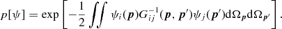 (6.5)
(6.5)
The Fourier transform  of the normalized density reads
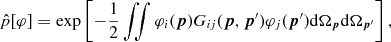 (6.6)
(6.6)
obtained by introducing a new integration variable  in the Fourier integral via the
shift
in the Fourier integral via the
shift  and by employing identity (6.2).
The n-point correlations are generated by
multiple differentiation of
and by employing identity (6.2).
The n-point correlations are generated by
multiple differentiation of  , using functional derivatives on
the unit sphere,
, using functional derivatives on
the unit sphere,  , with the spherical delta function
  . In this way, we find the Wick
expansion of the four-point function,
. In this way, we find the Wick
expansion of the four-point function,
 (6.7)
(6.7)
in products of the Green functions  , ia,
b = T, E,
B, …. If there is an odd number of factors, the
expectation value vanishes. The 2n-point function
is obtained by summing a product of n factors σab
over all unordered index pairs according to the pattern (6.7);
there are (2n)!/(n!2n)
summands.
, ia,
b = T, E,
B, …. If there is an odd number of factors, the
expectation value vanishes. The 2n-point function
is obtained by summing a product of n factors σab
over all unordered index pairs according to the pattern (6.7);
there are (2n)!/(n!2n)
summands.
We consider the Legendre-weighted average of the four-point correlation (6.7),
 (6.8)
(6.8)
which can be evaluated as
 (6.9)
(6.9)
Here, we used equations (6.3), (6.7) and the series representation (6.1) as well as the integral
 (6.10)
where the variables can be interchanged in pairs, p
i rightarrow
p j.
The integrations over the four unit spheres in equation (6.10)
are readily done by repeated application of the orthogonality relation
for Legendre polynomials in equation (2.6).
Weighted higher order correlations such as  are defined according to patterns (6.3)
and (6.8),
and can be expressed as linear combinations of products of multipole
coefficients analogous to equation (6.9).
are defined according to patterns (6.3)
and (6.8),
and can be expressed as linear combinations of products of multipole
coefficients analogous to equation (6.9).
We rename the indices in equation (6.9)
to i1, 2, 3, 4 = i,
j, m, n.
The covariance matrix 〈ΔCij;
lΔCmn;
k〉,  , thus reads
 (6.11)
which gives the cosmic variance  . The angle brackets refer to the
Gaussian functional (6.5)
and can formally be imagined as ensemble average over multiple copies
of the sky, with root mean squares σij;
l quantifying the fluctuations of the
coefficients Cij;
l.
This ensemble interpretation is borrowed from statistical mechanics,
but is less appealing here, as the ensemble and the average to which
the σij; l
refer are not realizable. The large error bars at low l,
cf. Figs 6 and 7,
are almost entirely due to cosmic variance (calculated via equation (6.11)
with
. The angle brackets refer to the
Gaussian functional (6.5)
and can formally be imagined as ensemble average over multiple copies
of the sky, with root mean squares σij;
l quantifying the fluctuations of the
coefficients Cij;
l.
This ensemble interpretation is borrowed from statistical mechanics,
but is less appealing here, as the ensemble and the average to which
the σij; l
refer are not realizable. The large error bars at low l,
cf. Figs 6 and 7,
are almost entirely due to cosmic variance (calculated via equation (6.11)
with  , as the measurement errors are very
small at low l as compared to σij;
l (Jarosik et al. 2011; Larson et al. 2011). The depicted error bars
obscure the fine structure of the low-l
power spectrum of the measured field configuration, the only accessible
one of the envisaged ensemble. Here, we have found an analytic Green
function for the temperature autocorrelation, which fits the power
spectrum within the actual measurement errors (rather than within the
error bars defined by the variance of a hypothetical ensemble average
over independent universes).
, as the measurement errors are very
small at low l as compared to σij;
l (Jarosik et al. 2011; Larson et al. 2011). The depicted error bars
obscure the fine structure of the low-l
power spectrum of the measured field configuration, the only accessible
one of the envisaged ensemble. Here, we have found an analytic Green
function for the temperature autocorrelation, which fits the power
spectrum within the actual measurement errors (rather than within the
error bars defined by the variance of a hypothetical ensemble average
over independent universes).
By identifying the pairs (ia,
p a)
in the four-point function (6.7),
one obtains contractions such as  , where σ11
and σ22 are constants and
, where σ11
and σ22 are constants and  is the squared two-point function (6.1)
depending on
is the squared two-point function (6.1)
depending on  . Correlations on large angular
scales, e.g. the weak temperature autocorrelation at
. Correlations on large angular
scales, e.g. the weak temperature autocorrelation at  (Bennett et al. 2011), are quantified by truncated
angular averages such as
(Bennett et al. 2011), are quantified by truncated
angular averages such as  , which can be evaluated by means of
the Legendre series (6.1)
and the uniform analytic approximation of the multipole coefficients
stated in Section 'RECONSTRUCTION
OF THE CMB TEMPERATURE POWER SPECTRUM'.
, which can be evaluated by means of
the Legendre series (6.1)
and the uniform analytic approximation of the multipole coefficients
stated in Section 'RECONSTRUCTION
OF THE CMB TEMPERATURE POWER SPECTRUM'.
7 CONCLUSION
- Top of page
- ABSTRACT
- 1 INTRODUCTION
- 2 CMB TEMPERATURE FLUCTUATIONS: GENERAL SETTING
- 3 MULTIPOLE MOMENTS OF ISOTROPIC GAUSSIAN RANDOM FIELDS ON THE UNIT SPHERE
- 4 RECONSTRUCTION OF THE CMB TEMPERATURE POWER SPECTRUM
- 5 MULTIPOLE FINE STRUCTURE OF CMB TEMPERATURE FLUCTUATIONS
- 6 OUTLOOK: MULTICOMPONENT SPHERICAL RANDOM FIELDS
- 7 CONCLUSION
- REFERENCES
- Appendix A
- Appendix B
We designed an analytic method to reconstruct correlation functions of spherical Gaussian random fields from measured power spectra. The isotropic correlations are defined by a Hermitian matrix kernel, composed of Gaussian power-law densities and Kummer distributions. We obtained a closed analytic expression for the CMB temperature autocorrelation function, fitted its kernel to the measured multipole spectrum and tested the quality of the fit in various intervals over an extended multipole range, cf. Figs 6-13. The multipole coefficients are obtained by averaging squared spherical Bessel functions with the matrix kernel of the Green function, cf. Section 'MULTIPOLE MOMENTS OF ISOTROPIC GAUSSIAN RANDOM FIELDS ON THE UNIT SPHERE'. In Tables 1 and 2, we list the fitting parameters of the distributions defining the spectral kernel. Once the kernel of the Green function is specified, so are all higher n-point correlations of the Gaussian random field.
The fine structure of the CMB temperature power spectrum in
the low-l
regime suggests that the Sachs–Wolfe ‘plateau’ precursory to the main
peak is a superposition of overlapping Gaussian peaks, shown in Figs 6
and 7 as
dashed curves. In contrast, the high-l power
spectrum above l ∼ 1000 consists of two
non-Gaussian oscillatory components (depicted in Figs 9-13
as dotted curves  and
and  generated by Kummer distributions,
cf. Table 2.
generated by Kummer distributions,
cf. Table 2.
The fine structure of CMB power spectra can be hidden in
compressed spectral plots as shown in Figs 1-5,
which give no more than an overview of the basic features of the
spectral map, and make it even difficult to identify the Gaussian and
transitional peaks and to discern them from periodic modulations. The
low-l regime up to l ∼ 400
is composed of Gaussian peaks, cf. Figs 6 and 7.
The two transitional peaks in the crossover region 400 ≤ l
≤ 1000, cf. Figs 8 and 9,
are mixtures of Gaussian peaks and large-amplitude modulations of the
Kummer distributions. The intermediate and high-l
multipole regimes in Figs 12 and 13
comprise a modulated decaying slope  and a rising power-law slope
  stemming from the Kummer
distributions in the spectral kernel of the correlation function.
stemming from the Kummer
distributions in the spectral kernel of the correlation function.
Hermitian spectral matrices are an efficient analytic tool to reconstruct correlation functions of spherical Gaussian random fields from angular power spectra. Here, we studied the CMB temperature autocorrelation, based on a multipole spectrum measured up to l ∼ 104, cf. Fig. 1. Other applications are CMB polarization correlations and temperature–polarization cross-correlations, or galaxy angular correlations. In all these cases, the multipole expansion of the spherical Green function is a Legendre series in zonal spherical harmonics due to isotropy, cf. Section 'OUTLOOK: MULTICOMPONENT SPHERICAL RANDOM FIELDS', so that the correlation functions can be reconstructed from the measured (cross-)power spectra as described in Sections 'MULTIPOLE MOMENTS OF ISOTROPIC GAUSSIAN RANDOM FIELDS ON THE UNIT SPHERE' and 'RECONSTRUCTION OF THE CMB TEMPERATURE POWER SPECTRUM'.
REFERENCES
- Top of page
- ABSTRACT
- 1 INTRODUCTION
- 2 CMB TEMPERATURE FLUCTUATIONS: GENERAL SETTING
- 3 MULTIPOLE MOMENTS OF ISOTROPIC GAUSSIAN RANDOM FIELDS ON THE UNIT SPHERE
- 4 RECONSTRUCTION OF THE CMB TEMPERATURE POWER SPECTRUM
- 5 MULTIPOLE FINE STRUCTURE OF CMB TEMPERATURE FLUCTUATIONS
- 6 OUTLOOK: MULTICOMPONENT SPHERICAL RANDOM FIELDS
- 7 CONCLUSION
- REFERENCES
- Appendix A
- Appendix B
- et al., 2011, ApJS, 192, 17
- et al., 2009, ApJ, 705, 978
- et al., 2011, ApJ, 729, 62
- , 1999, Classical Electrodynamics, 3rd edn. Wiley, New York
- et al., 2011, ApJS, 192, 14
- , 1923, Proc. R. Soc. A, 102, 554
- et al., 2006, ApJ, 647, 823
- et al., 2011, ApJ, 743, 28
- , , 1991, Quantum Mechanics: Non-Relativistic Theory, 3rd edn. Pergamon, London
- et al., 2011, ApJS, 192, 16
- , , , 1966, Formulas and Theorems for the Special Functions of Mathematical Physics. Springer, New York
- et al., 2010, J. Phys. G, 37, 075021, http://pdg.lbl.gov
- , 1982, Scattering Theory of Waves and Particles. Springer, New York
- , , , , 2010, NIST Handbook of Mathematical Functions. Cambridge Univ. Press, Cambridge, http://dlmf.nist.gov
- et al., 2009, ApJ, 694, 1200
- et al., 2012, ApJ, 755, 70
- et al., 2009, preprint (arXiv:0901.4540)
- , 2012, Europhys. Lett., 97, 39003
Appendix A
- Top of page
- ABSTRACT
- 1 INTRODUCTION
- 2 CMB TEMPERATURE FLUCTUATIONS: GENERAL SETTING
- 3 MULTIPOLE MOMENTS OF ISOTROPIC GAUSSIAN RANDOM FIELDS ON THE UNIT SPHERE
- 4 RECONSTRUCTION OF THE CMB TEMPERATURE POWER SPECTRUM
- 5 MULTIPOLE FINE STRUCTURE OF CMB TEMPERATURE FLUCTUATIONS
- 6 OUTLOOK: MULTICOMPONENT SPHERICAL RANDOM FIELDS
- 7 CONCLUSION
- REFERENCES
- Appendix A
- Appendix B
DELTA FUNCTION AND LEGENDRE EXPANSION ON THE UNIT SPHERE
The delta function  on the unit sphere
  can be defined by
  , where
  is the solid-angle element with
polar axis n, and f(n)
is an arbitrary smooth and square-integrable function on the unit
sphere. Thus,
is the solid-angle element with
polar axis n, and f(n)
is an arbitrary smooth and square-integrable function on the unit
sphere. Thus,  , with δ(cos θ − cos θ′) = δ(θ −
θ′)/sin θ, where the angles (θ, ϕ) and (θ′, ϕ′) are the polar
coordinates of the unit vectors n
and
, with δ(cos θ − cos θ′) = δ(θ −
θ′)/sin θ, where the angles (θ, ϕ) and (θ′, ϕ′) are the polar
coordinates of the unit vectors n
and  .
.
Spherical harmonics Ylm(θ,
ϕ) are denoted by Ylm(n),
where  is a unit vector in polar
coordinates. The Ylm(θ,
ϕ), l = 0, 1, 2…, −l ≤ m
≤ l, are complete on the unit sphere; their
orthogonality and completeness relations (Olver et al. 2010) read in this notation
is a unit vector in polar
coordinates. The Ylm(θ,
ϕ), l = 0, 1, 2…, −l ≤ m
≤ l, are complete on the unit sphere; their
orthogonality and completeness relations (Olver et al. 2010) read in this notation
 (A1)
(A1)
 (A2)
(A2)
and we use the normalizations  and
and  .
Isotropic spherical random fields can be expanded in Legendre
polynomials or zonal harmonics, which constitute a complete orthogonal
set over the interval −1 ≤ x ≤ 1, with the
orthogonality and completeness relations
.
Isotropic spherical random fields can be expanded in Legendre
polynomials or zonal harmonics, which constitute a complete orthogonal
set over the interval −1 ≤ x ≤ 1, with the
orthogonality and completeness relations
 (A3)
(A3)
 (A4)
(A4)
A square-integrable function f(x) on the interval [−1, 1] admits the expansion
 (A5)
(A5)
If we put  , we find the Legendre expansion of
the isotropic field f(n
k 0) on
the sphere
, we find the Legendre expansion of
the isotropic field f(n
k 0) on
the sphere  as
as
 (A6)
(A6)
The multipole coefficients Cl are independent of the arbitrarily chosen unit vector k 0. We also note P0(x) = 1, Pl(1) = 1, as well as the reflection symmetry Pl(x) = (−1)lPl(−x). This expansion can be traced back to spherical harmonics via the addition theorem (Newton 1982; Jackson 1999)
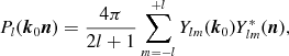 (A7)
(A7)
where we may interchange k 0 and n. Combining equation (A7) with the completeness relation for spherical harmonics (A2), we find the Legendre series of the delta function on the unit sphere as stated in equation (2.13).
We consider isotropic spherical random fields (depending only
on the polar angle θ), so that Legendre expansions of type (A6)
in zonal harmonics  suffice. We note
  , where
  is the Laplace–Beltrami operator on
the unit sphere (Landau & Lifshitz 1991). The high-l
asymptotics
is the Laplace–Beltrami operator on
the unit sphere (Landau & Lifshitz 1991). The high-l
asymptotics
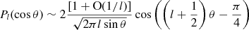 (A8)
(A8)
can be used to identify the wavelength  on the unit sphere (Jeans 1923). This gives an estimate of the
angular resolution achieved by high-order multipole moments in the
Legendre expansion (2.27)
of the two-point function
on the unit sphere (Jeans 1923). This gives an estimate of the
angular resolution achieved by high-order multipole moments in the
Legendre expansion (2.27)
of the two-point function  , where we put
  .
.
Appendix B
- Top of page
- ABSTRACT
- 1 INTRODUCTION
- 2 CMB TEMPERATURE FLUCTUATIONS: GENERAL SETTING
- 3 MULTIPOLE MOMENTS OF ISOTROPIC GAUSSIAN RANDOM FIELDS ON THE UNIT SPHERE
- 4 RECONSTRUCTION OF THE CMB TEMPERATURE POWER SPECTRUM
- 5 MULTIPOLE FINE STRUCTURE OF CMB TEMPERATURE FLUCTUATIONS
- 6 OUTLOOK: MULTICOMPONENT SPHERICAL RANDOM FIELDS
- 7 CONCLUSION
- REFERENCES
- Appendix A
- Appendix B
EULER PARAMETRIZATION OF HERMITIAN SPECTRAL MATRICES
We consider a positive semidefinite Hermitian 3 × 3 matrix gmn, cf. (3.1), which we decompose as
 (B1)
(B1)
with real diagonal coefficients aj ≥ 0, analogous to the two-dimensional case in equations (3.3) and (3.4). Positive definiteness requires aj > 0. The matrices Ri(θi, ψi, χi), i = 1, 2, 3, in equation (B1) denote SU(3) subgroups composed of the SU(2) matrices
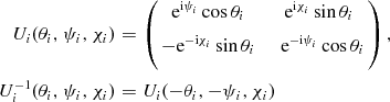 (B2)
(B2)
in the following way:
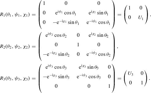 (B3)
(B3)
The inverse matrices in the decomposition (B1) are found as
 (B4)
(B4)
If we put ψi = χi
= 0, i = 1, 2, 3, then the product R1(θ1)R2(−θ2)R3(θ3)
is a classical Euler parametrization of the rotation group SO(3), with  and
and  . In this case, the Hermitian gmn
in equation (B1)
is real and symmetric. Here, we do not impose any restrictions on the
angles θi, χi
and ψi other than reality.
. In this case, the Hermitian gmn
in equation (B1)
is real and symmetric. Here, we do not impose any restrictions on the
angles θi, χi
and ψi other than reality.
In N dimensions, the Euler parametrization of a Hermitian matrix gmn, m, n = 0, … , N − 1, is performed in like manner,
 (B5)
(B5)
with three-parameter subgroups Ri(θi,
ψi, χi),
i = 1, … , N(N
− 1)/2, of SU(N), each of them defined by an SU(2)
matrix inserted into an N × N
identity matrix according to the pattern (B3).
In this way, the matrices gmn
are parametrized by N2
independent real parameters, (aj
≥ 0, θi, ϕi),
j = 1, … , N and i
= 1, … , N(N − 1)/2, where ϕi
can be chosen as linear combinations of the N(N
− 1) angles ψi and χi
of the SU(N) subgroups Ri(θi,
ψi, χi).
For the amplitudes and angles, we use a spectral parametrization (aj(k),
θi(k),
ϕi(k))
analogous to equations (3.15)
and (3.16),
that is, a linear or quadratic k dependence of
the angles, and Gaussian power-law densities as amplitudes.
three-parameter subgroups Ri(θi,
ψi, χi),
i = 1, … , N(N
− 1)/2, of SU(N), each of them defined by an SU(2)
matrix inserted into an N × N
identity matrix according to the pattern (B3).
In this way, the matrices gmn
are parametrized by N2
independent real parameters, (aj
≥ 0, θi, ϕi),
j = 1, … , N and i
= 1, … , N(N − 1)/2, where ϕi
can be chosen as linear combinations of the N(N
− 1) angles ψi and χi
of the SU(N) subgroups Ri(θi,
ψi, χi).
For the amplitudes and angles, we use a spectral parametrization (aj(k),
θi(k),
ϕi(k))
analogous to equations (3.15)
and (3.16),
that is, a linear or quadratic k dependence of
the angles, and Gaussian power-law densities as amplitudes.