Nonlinear multiparametric modeling of life-table data with adaptive distributions: time evolution of hazard ratios

Abstract

Factorizing multiparameter densities are proposed for the analytic continuum modeling of human life tables. The formalism is developed based on mortality data of the female, male, and total population of France for the year 2021. The data sets cover the age range from birth up to 110 years. The cumulative hazard function is a multiply broken exponential density, admitting a differential hazard rate capable of describing the observed late-life mortality deceleration and exhibiting exponential asymptotic increase rather than a mortality plateau. The nonlinear least-squares regression is performed with the survival function, which admits double-exponential decay in the high-age limit. The minimization of the multiparametric least-squares functional is facilitated by invoking the product structure of the cumulative hazard, the number of factors and fitting parameters being adapted to the data set. More generally, new techniques are developed to deal with probability densities exhibiting a nonlinear multiparameter dependence. Such densities are increasingly needed to represent extended data sets, as exemplified by recent mortality data across the tree of life. In the case of the mentioned human life tables, the residual deviations of the regressed survival functions and cumulative distributions from the data points are within at most two percent, uniformly over the entire empirical age range. The analytic probability density and age-conditioned survival probabilities are calculated for the total population and the female and male cohorts. The lifetime evolution of the cumulative and differential female/male hazard ratios is studied, from birth up to the asymptotic high-age regime.

1 Introduction

The aim is to introduce analytic survival functions capable of representing life-table data over the entire age range and to develop methods to effectively cope with the nonlinear multiparameter dependence of these densities in the least-squares regression. The suggested distributions will be put to test with the life tables of France for the year 2021, cf. Ref. [1].

Commonly employed distributions for life tables such as logistic, Gompertz–Makeham and Weibull densities, cf., e.g., Refs. [2, 3], or distributions based on the assumption of population heterogeneity (frailty models [4, 5]) typically depend on two to four parameters. These densities can only describe limited sections of the empirical age range, for instance, the intermediate regime in the interval between around 40 years and the median lifetime (Gompertz–Makeham) or putative mortality plateaus, that is, asymptotically constant hazard rates (aka mortality or death rates) in the supercentenarian regime above 110 years (logistic and frailty models). Partial life-table modeling with the mentioned distributions has been discussed in the above quoted reviews.

We will focus on life-table data in the well-documented age range of below 110 years, cf. Ref. [1], and make use of the fact that the multiparametric densities introduced in this paper also allow extrapolation of the survival functions and mortality rates to the supercentenarian regime. The formalism of multiparameter survival functions will be developed from scratch. The figure and table captions are rather detailed, so that one can get an overview by starting with them.

A substantial part of this paper deals with the nonlinear least-squares regression of multiparameter survival functions $S(t)$, globally over the entire empirical lifetime range. In the case of the French life tables studied here, this means from birth ($t = 0$) up to an age of 110 years. In this time range, the survival function, which is a monotonically decreasing function normalized to one at $t = 0$, varies over four logarithmic decades. We will explain how to find an analytic fit to the survival data with a residual deviation from the data set of less than one or at most two percent, uniformly over the entire data range.

The cumulative distribution function can, in principle, be calculated from the survival function as $F(t) = 1 - S(t)$. However, a residual relative error of below one percent for $F(t)$ fitted to the cumulative data points cannot be maintained in this way, since $F(t)$ converges to zero at low age, whereas the survival function converges to one. To achieve this accuracy for both the survival function and, consistently, also for the cumulative density, we will perform a simultaneous least-squares fit of $S(t)$ and $F(t)$. The least-squares functional to be minimized in this context has a nonlinear multiparameter dependence, and a major topic of this paper will be the variational minimization of this functional. (In contrast, simultaneous least-squares regression is not needed for the Weibull or logistic or Gompertz survival function [2,3,4] and corresponding cumulative density, since these distributions cannot be used for the low-age regime of life tables anyway, and the same holds true for the survival functions of frailty models [5].)

Once an accurate analytic representation of the survival function $S(t)$ and cumulative distribution $F(t)$ has been found, one can calculate the associated probability density (pdf) $f(t) = F^{\prime}(t)$ and hazard rate $h(t) = f(t)/S(t)$ (force of mortality), the latter being the derivative of the cumulative hazard function $H(t) = - \log S(t)$. These distributions are also plotted in the figures, for the total population as well as for the female and male cohorts. The ratio of the female and male hazard rates and of the female and male cumulative hazards allows us to compare the mortality of different cohorts as a function of lifetime.

The basic functions $S(t)$, $F(t)$, $f(t)$, $h(t)$ and $H(t)$ of survival analysis are equivalent in the sense that knowledge of one of them suffices to calculate the remaining four. The question then arises as to which of these functions can most efficiently be regressed from the respective data set. In the case of life tables, the data sets for the pdf $f(t)$ and hazard rate $h(t)$ are obtained by finite difference approximations from the tabulated data of the survival function $S(t)$, resulting in loss of accuracy; the data sets of $f(t)$ and $h(t)$ are plotted in the figures to illustrate this. In contrast, the data sets of the cumulative distribution $F(t)$ and cumulative hazard function $H(t)$ can be obtained without approximations from the survival data. The cumulative hazard $H(t)$ is found by taking the logarithm of the ordinate of the survival data points, leading to a compressed data range in the least-squares functional, which is also detrimental to accuracy, cf. Section 3. Therefore, we will add the least-squares functionals of $S(t)$ and $F(t)$ and minimize the combined nonlinear functional, taking into account the relation of $S(t)$ and $F(t)$, as pointed out above.

The multiply broken exponential distributions employed as cumulative hazard functions (see below and Sect. 2 for definitions) do not result in asymptotically constant hazard rates like logistic and frailty models [2, 4,5,6], but rather in double-exponentially decaying survival functions and exponentially increasing mortality rates similar to the Gompertz density [3]. As mentioned, the multiparameter densities introduced in this paper are applicable over the entire age range, whereas the Gompertz or Gompertz–Makeham densities [3] are designed for the intermediate and high age regime. We will also demonstrate that the deceleration of the high-age mortality rate [6] clearly visible in the data sets depicted in the figures can accurately be described with multiply broken exponential distributions. The residual deviations of the cumulative hazard function $H(t)$ from the data points are below two percent. The slightly decelerating hazard rate below the age of 110 years does not terminate in a mortality plateau in the supercentenarian regime, the extrapolated hazard rate increasing exponentially; see also Sect. 6 for more discussion on that. The regression technique of multiparametric survival functions with nonlinear parameter dependence developed here and put to test by analyzing data sets of human life tables can also be applied to mortality data of other mammalian species, cf. Section 6.

In Sect. 2, we will introduce the multiply broken exponential densities defining the cumulative hazard function, which factorize as $H(t) = a_{0} t^{{\alpha_{0} }} \prod\nolimits_{k = 0}^{n} {(1 + {\text{e}}^{{(\beta_{k} /\left| {\eta_{k} } \right|)(t - b_{k} )}} )^{{\eta_{k} }} }$, analogously to the broken power laws in Refs. [7,8,9]. The factor $a_{0} t^{{\alpha_{0} }}$ describes the initial increase in the low-age regime and the factors $(1 + {\text{e}}^{{(\beta_{k} /\left| {\eta_{k} } \right|)(t - b_{k} )}} )^{{\eta_{k} }}$ (with positive parameters $\beta_{k}^{{}}$, $b_{k}^{{}}$ and nonzero exponent $\eta_{k}^{{}}$) determine the exponential increase in the intermediate and high-age range. The exponential factors resemble Fermi distributions for negative exponents $\eta_{k}^{{}}$, cf., e.g., Ref. [10], and have similar limit (cutoff) properties explained in Sect. 2. The number of exponential factors required in the above product depends on the data set and data range available for regression. The survival function is obtained by exponentiation of the cumulative hazard, $S(t) = \exp ( - H(t))$, admitting double-exponential decay. In Sect. 2, we will also sketch the logarithmic representation of the data sets and the parameters defining the cumulative hazard $H(t)$.

In Sect. 3, the nonlinear least-squares regression of the survival function and cumulative distribution is explained. Since $S(t)$ and $F(t)$ differ in their order of magnitude both in the high- and low-age regimes, we perform a simultaneous fit of these functions with a properly weighted least-squares functional, to obtain uniformly accurate fits of $S(t)$ and $F(t)$ over the empirical age range. As $S(t)$ and $F(t)$ are multiparameter distributions with nonlinear parameter dependence, the minimization of the least-squares functional, cf., e.g., Refs. [11,12,13,14,15,16,17], requires reasonably accurate initial values for the parameters. The estimation of initial values by successively fitting the factors of $H(t)$ to the data set in Log–Lin representation is also explained in Sect. 3. The uniform accuracy of the regressed distributions is quantified by residual panels in the figures and by goodness-of-fit parameters.

In Sect. 4, the differential hazard rate $h(t)$ and lifetime probability density $f(t)$ are discussed, both of which are calculated from the regressed analytic survival function $S(t)$ by differentiation. We also briefly explain how to obtain data points for these distributions from the data set of $S(t)$ by finite difference methods. Age-conditioned survival probabilities and differential and cumulative hazard ratios are also outlined in this section.

In Sect. 5, the factorizing cumulative hazard functions $H(t)$ are put to test with mortality data of the female and male cohorts and the total population of France for the year 2021. The regressed survival function $S(t)$, cumulative distribution $F(t)$, cumulative hazard function $H(t)$, pdf $f(t)$ and differential hazard rate $h(t)$ are depicted in Figs. 1, 2, 3, 4, 5 for the total population, in Figs. 6, 7, 8, 9 for females and in Figs. 10, 11, 12, 13 for the male cohort. The lifetime evolution of the cumulative and differential hazard ratios H_♀(t)/H_♂(t) and h_♀(t)/h_♂(t) of the female and male population is plotted in Fig. 14. The regressed parameters and goodness-of-fit parameters are recorded in Table 1 for the respective population. Table 2 lists hazard rates and age-conditioned survival probabilities at selected ages. Median lifetimes derived from the regressed survival functions are reported in the captions of Figs. 1, 6, 10. In Sect. 6, we discuss future research directions regarding non-human life tables.

Fig. 1

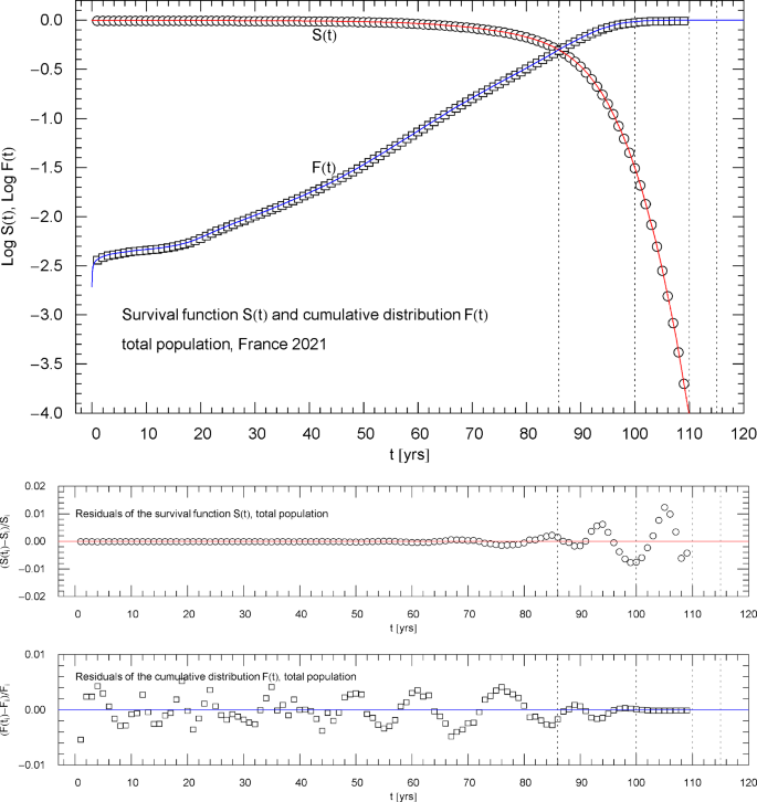
Survival function $S(t)$ and cumulative distribution $F(t)$ of the 2021 total population of France. Data points from Ref. [1]. The intersection point of the two curves defines the median lifetime t_m = 85.98 year. The least-squares fit is performed with $S(t) = \exp ( - H(t))$, where $H(t)$ is the multiply broken exponential distribution (2.1) (cumulative hazard) with regressed parameters in Table 1. The least-squares functional defining the simultaneous fit of $S(t)$ and $F(t)$ is stated in (3.2). The abscissas of the dotted vertical lines are located at $t = t_{{\text{m}}} , \, 100, \, 110, \, 115{\text{ yrs}}$. The lower panels show the residuals of the regressed functions $S(t)$ and $F(t)$ with respect to the data points

Fig. 2

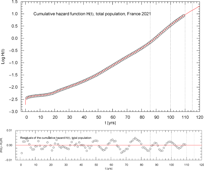
Cumulative hazard function $H(t)$ of the 2021 total population of France. The depicted data points were extracted from the data set of the survival function [1], cf. Section 2. The cumulative hazard function (red solid curve) is the broken exponential distribution $H(t) = - \log S(t)$, cf. (2.1) and Table 1, obtained from the regressed survival function $S(t)$ in Fig. 1. The dotted vertical lines are located at $t = t_{{\text{m}}} , \, 100, \, 110, \, 115{\text{ yrs}}$. ($t_{{\text{m}}}$ denotes the median lifetime, cf. the end of Sect. 3 and Fig. 1.) The lower panel shows the residuals of the regressed $H(t)$ with respect to the data points

Fig. 3

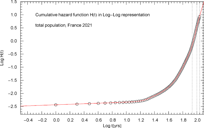
Cumulative hazard function $H(t)$ of the 2021 total population of France. Depicted is the same data set and regressed curve $H(t)$ as in Fig. 2, but now in Log–Log coordinates, where the low-age slope appears as straight line representing the asymptotic power law $H(t)\sim at^{{\alpha_{0} }}$, cf. after (2.1). The dotted vertical lines are located at $t = t_{{\text{m}}} , \, 100, \, 110, \, 120{\text{ yrs}}$. ($t_{{\text{m}}} = 85.98{\text{ yr}}$ is the median lifetime)

Fig. 4

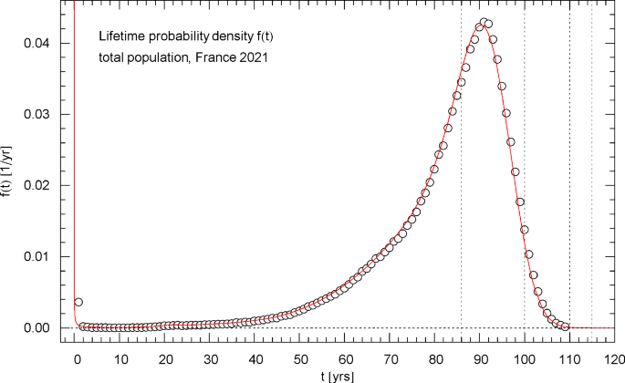
Lifetime probability density of the 2021 total population of France. The data points were calculated from the data set of the survival function in Fig. 1 by way of a finite-difference approximation, cf. Section 4. The red solid curve depicts the probability density $f(t) = F^{\prime}(t)$, obtained from the regressed cumulative distribution in Fig. 1. $f(t)$ diverges at $t = 0$ but stays integrable (since $F(t) \propto t^{{\alpha_{0} }}$, $0 < \alpha_{0} < 1$, in this limit, cf. Table 1) and is normalized to one. The first of the vertical dotted lines indicates the median lifetime $t_{{\text{m}}} = 85.98{\text{ yr}}$, the other lines are located at 100, 110 and 115 years. The density attains its maximum at the modal age $t_{{{\text{max}}}} = 90.36{\text{ yr}}$

Fig. 5

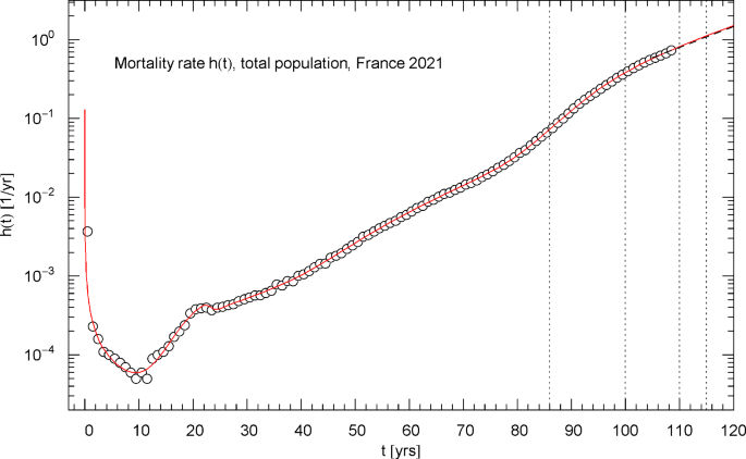
Mortality rate (hazard rate) of the 2021 total population of France. The data points were calculated from the survival data in Fig. 1 as finite differences, cf. Section 4. The red solid curve depicts the mortality rate $h(t) = H^{\prime}(t)$, cf. (4.1), obtained from the regressed cumulative hazard in Fig. 2. In the high-age limit, $h(t)$ increases exponentially, cf. (4.2). (Simple exponential increase appears as straight line in the Log–Lin coordinates of this figure.) The low-age limit is a singular power law, $h(t)\sim a\alpha_{0} t^{{\alpha_{0} - 1}}$, cf. after (2.1) and Table 1. The first of the vertical dotted lines indicates the median lifetime $t_{{\text{m}}} = 85.98{\text{ yr}}$. The minimum of the mortality rate is attained at $t_{{{\text{min}}}} = 9.41{\text{ yr}}$. Also indicated as black dashed straight line starting at $t = {\text{ 105 yr}}$ is the Gompertz hazard function regressed in Ref. [41] from survival data in the 105–115 yr range

Fig. 6

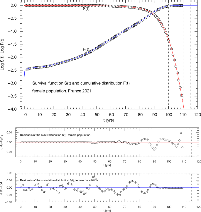
Survival function $S(t)$ and cumulative distribution $F(t)$ of the 2021 female population of France. Data points from Ref. [1]. The intersection point of the two curves defines the median lifetime $t_{{\text{m}}} = 88.52{\text{ yr}}$. The least-squares fit, cf. Section 3, is performed with $S(t) = \exp ( - H(t))$, where $H(t)$ is the multiply broken exponential distribution (2.1) (cumulative hazard function) with regressed parameters in Table 1. The abscissas of the dotted vertical lines are located at $t = t_{{\text{m}}} , \, 100, \, 110, \, 115{\text{ yrs}}$. The lower panels show the residuals of the regressed functions $S(t)$ and $F(t)$ with respect to the data points

Fig. 7

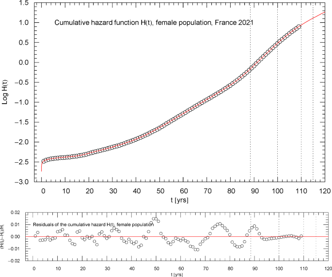
Cumulative hazard function $H(t)$ of the 2021 female population of France. The depicted data points were extracted from the data set of the survival function, cf. Section 2. The cumulative hazard (red solid curve) is the broken exponential distribution $H(t) = - \log S(t)$, cf. (2.1) and Table 1, calculated from the regressed survival function $S(t)$ in Fig. 6. The dotted vertical lines are located at $t = t_{{\text{m}}} , \, 100, \, 110, \, 115{\text{ yrs}}$. ($t_{{\text{m}}}$ denotes the median lifetime, cf. Figure 6.) The lower panel shows the residuals of the regressed $H(t)$ with respect to the data points

Fig. 8

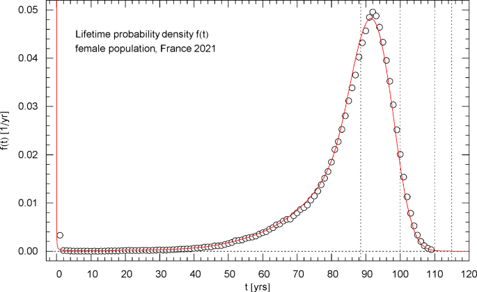
Lifetime probability density of the 2021 female population of France. The data points were calculated from the data set of the survival function in Fig. 6 via a finite-difference approximation, cf. Section 4. The red solid curve depicts the probability density $f(t) = F^{\prime}(t)$, obtained from the regressed cumulative distribution in Fig. 6. $f(t)$ diverges at $t = 0$ but stays integrable (since $F(t) \propto t^{{\alpha_{0} }}$, $0 < \alpha_{0} < 1$, in this limit, cf. Table 1) and is normalized to one. The first of the vertical dotted lines indicates the median lifetime $t_{{\text{m}}} = 88.52{\text{ yr}}$. The density attains its maximum at the modal age $t_{{{\text{max}}}} = 91.47{\text{ yr}}$

Fig. 9

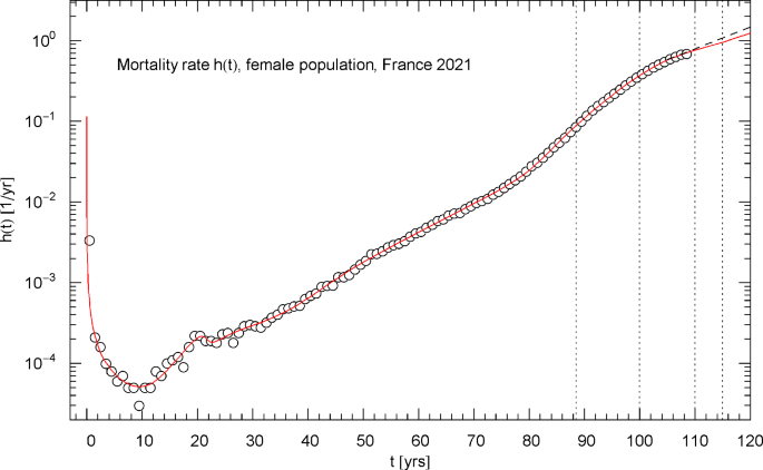
Mortality rate of the 2021 female population of France. The data points were calculated from the survival data in Fig. 6 as finite differences, cf. Section 4. The red solid curve depicts the mortality rate $h(t) = H^{\prime}(t)$, cf. (4.1), obtained from the regressed cumulative hazard in Fig. 7. In the asymptotic high-age limit, $h(t)$ increases exponentially, cf. (4.2). The low-age limit is a singular power law, $h(t)\sim a\alpha_{0} t^{{\alpha_{0} - 1}}$, cf. after (2.1) and Table 1. The first of the vertical dotted lines indicates the median lifetime $t_{{\text{m}}} = 88.52{\text{ yr}}$. The minimum of the mortality rate is attained at $t_{{{\text{min}}}} = 9.52{\text{ yr}}$. Also indicated as black dashed straight line starting at $t = {\text{ 105 yr}}$ is the Gompertz hazard function regressed in Ref. [41] from survival data in the 105–115 yr range

Fig. 10

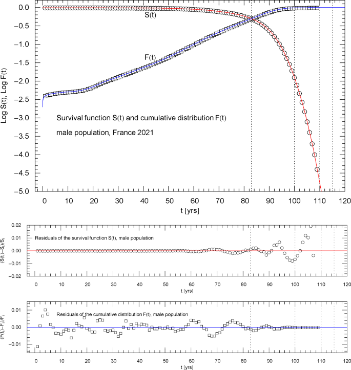
Survival function $S(t)$ and cumulative distribution $F(t)$ of the 2021 male population of France. Data points from Ref. [1]. The intersection point of the two curves defines the median lifetime $t_{{\text{m}}} = 82.91{\text{ yr}}$. The least-squares fit, cf. Section 3, is performed with $S(t) = \exp ( - H(t))$, where $H(t)$ is the multiply broken exponential distribution (2.1) (cumulative hazard) with regressed parameters in Table 1. The abscissas of the dotted vertical lines are located at $t = t_{{\text{m}}} , \, 100, \, 110, \, 115{\text{ yrs}}$. The lower panels show the residuals of the regressed functions $S(t)$ and $F(t)$ with respect to the data points

Fig. 11

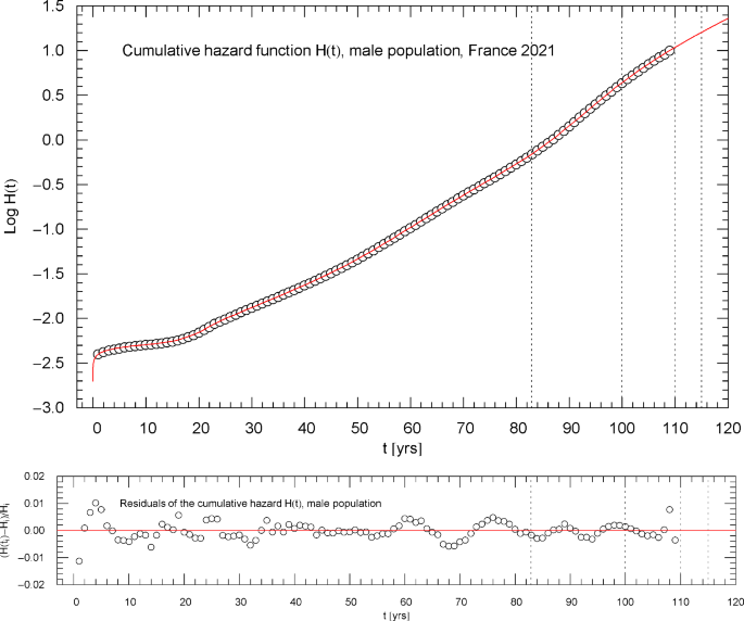
Cumulative hazard function $H(t)$ of the 2021 male population of France. The depicted data points were extracted from the data set of the survival function, cf. Section 2. The cumulative hazard (red solid curve) is the broken exponential density $H(t) = - \log S(t)$, cf. (2.1) and Table 1, obtained from the regressed survival function $S(t)$ in Fig. 10. The dotted vertical lines are located at $t = t_{{\text{m}}} , \, 100, \, 110, \, 115{\text{ yrs}}$. ($t_{{\text{m}}}$ denotes the median lifetime, cf. Figure 10.) The lower panel shows the residuals of the regressed $H(t)$ with respect to the data points

Fig. 12

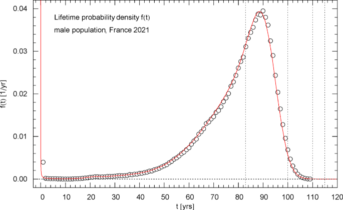
Lifetime probability density of the 2021 male population of France. The data points were calculated from the data set of the survival function in Fig. 10 by way of a finite-difference approximation, cf. Section 4. The red solid curve depicts the probability density $f(t) = F^{\prime}(t)$, obtained from the regressed cumulative distribution in Fig. 10. $f(t)$ diverges at $t = 0$ but stays integrable (since $F(t) \propto t^{{\alpha_{0} }}$, $0 < \alpha_{0} < 1$, in this limit, cf. Table 1) and is normalized to one. The first of the vertical dotted lines indicates the median lifetime $t_{{\text{m}}} = 82.91{\text{ yr}}$. The density attains its maximum at the modal age $t_{{{\text{max}}}} = 88.57{\text{ yr}}$

Fig. 13

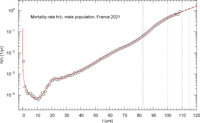
Mortality rate (hazard rate) of the 2021 male population of France. The data points were calculated from the survival data in Fig. 10 as finite differences, cf. Section 4. The red solid curve depicts the mortality rate $h(t) = H^{\prime}(t)$, cf. (4.1), obtained from the regressed cumulative hazard in Fig. 11. In the asymptotic high-age limit, $h(t)$ increases exponentially, cf. (4.2). The low-age limit is a singular power law, $h(t)\sim a\alpha_{0} t^{{\alpha_{0} - 1}}$, cf. after (2.1) and Table 1. The first of the vertical dotted lines indicates the median lifetime t_m=82.91 year. The minimum of the mortality rate is attained at t_min = 9.48 year. Also indicated as black dashed straight line starting at t=105 year is the Gompertz hazard function regressed in Ref. [41] from survival data in the 105–115 yr range

Fig. 14

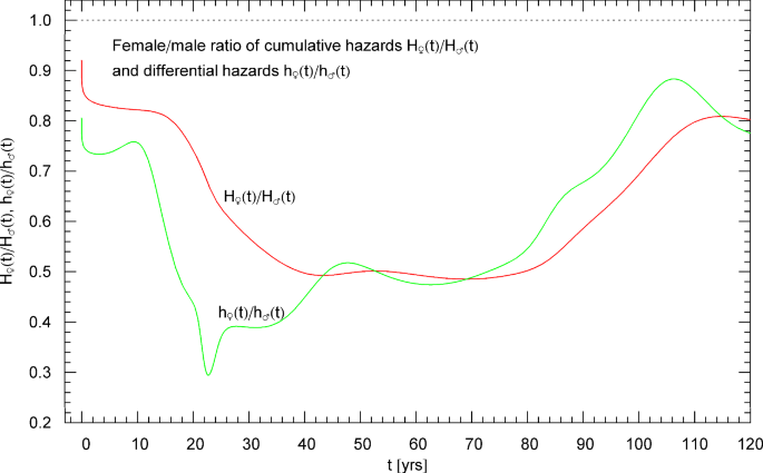
Time evolution of the differential hazard ratio h_♀(t)/h_♂(t) (green curve) and cumulative hazard ratio H_♀(t)/H_♂(t) (red curve) of the female and male population of France, based on the 2021 life tables. The regressed female and male hazard rates h_♀(t) and h_♂(t) are depicted in Figs. 9 and 13 and the cumulative hazards H_♀(t) and H_♂(t) in Figs. 7 and 11. At an age of around 23 years, a pronounced dip is visible in the h_♀(t)/h_♂(t) curve of the differential hazards, due to an elevated accident rate in the male juvenile population. The depicted ratios stay below one over the entire age range, the male mortality being consistently higher than the female one

Table 1 Fitting parameters of the survival functions of the 2021 total/female/male population of France, cf. Ref. [1]

Table 2 Survival function $S(t)$, hazard rate $h(t)$, and probability $p_{ + 1} (t) = S(t + 1)/S(t)$ to live one further year conditional upon survival up to age $t$, cf. Section 4

Finally, in the last half-century, nonlinear modeling has become a standard tool in a variety of research fields. Recent advances include nonlinear wave propagation in optical media [18], solitons in plasmas and fluids [19,20,21,22], surface and shallow-water waves [23,24,25,26,27], solitons in electrical lattices [28], and wave propagation in blood vessels [29] and through layered liquids [30]. Nonlinear fractional modeling has been applied to dissipative chaotic systems [31], agricultural production processes [32], ecological systems [33], permafrost thaw [34], and to electrical signal transfer [35]. Here, we add a new interdisciplinary research area where nonlinear empirical modeling is effective, that is mortality and senescence, surely a topic of general interest to mortals.

2 Multiply broken exponential distributions in survival analysis

In this section, we introduce the multiparameter distributions that will be used to model the mortality data analyzed in Sect. 5. As mentioned in the Introduction, standard distributions commonly employed in the literature, cf., e.g., Refs. [1,2,3,4,5], can only represent limited age ranges of life tables, and more adaptable distributions are needed to accurately represent mortality data over the full empirical lifetime range. By the way, the applicability of the multiply broken exponential distributions defined in (2.1) is not restricted to mortality data, human or otherwise, cf. Section 6, as the time variable can be replaced by other observables like temperature, energy, density, pressure, etc. The distributions defined in (2.1) have a genuinely nonlinear parameter dependence; linearization in any of the parameters is not an option, given that the time variable is unconstrained apart from positivity. An essential part of this paper is to develop variational least-squares techniques suitable for the nonlinear multiparameter dependence of the distributions (2.1) in real-world applications, which will be done in this and the subsequent section. But first we briefly sketch some basic properties of survival functions and associated distributions (to make this paper self-contained) as well as the notation used for the data sets defining them.

In Sect. 5, we will study the 2021 life tables of the female, male, and total population of France. The data sets defining the survival function $S(t)$ in 1-year increments from birth to 109 years are taken from Ref. [1]. The data points of the survival function $S(t)$ will be labeled $(t_{i} ,S_{i} )_{i = 1,...,N}$, with $t_{j} [{\text{yr}}] = j$, $j = 0,1,...,N$, $N = 109$, and $(t_{0} ,S_{0} ) = (0,1)$.

The data sets of the cumulative distribution $F(t)$ and cumulative hazard function $H(t)$ are obtained from the survival data $(t_{i} ,S_{i} )_{i = 1,...,N}$. Data points of $F(t)$ are denoted by $(t_{i} ,F_{i} )_{i = 1,...,N}$, where $F_{i} = 1 - S_{i}$, $(t_{0} ,F_{0} ) = (0,0)$, and data points of $H(t)$ by $(t_{i} ,H_{i} )_{i = 1,...,N}$, $H_{i} = - \log S_{i}$, and $(t_{0} ,H_{0} ) = (0,0)$. Apart from the distributions $S(t)$, $F(t)$ and $H(t)$, we will also derive, from the regressed survival function, the probability distribution $f(t)$ and the differential hazard rate $h(t)$ for the female, male, and total population, cf. Section 4.

The analytic distributions $S(t)$, $F(t)$, $H(t)$ are related by $F(t) = 1 - S(t)$ and $H(t) = - \log S(t)$, where $S(t)$ is monotonically decreasing from $S(0) = 1$ to zero, $S(t \to \infty ) = 0$, admitting exponential decay (specified below). Accordingly, $H(t)$ is monotonically increasing from zero to infinity and $F(t)$ from zero to one. Since $H(t) = - \log (1 - F(t))$, we have $H(t)\sim F(t)$ in the short-time (low age) regime.

The pdf $f(t)$ is the negative derivative of the survival function, $f(t) = - S^{\prime}(t)$, and the differential hazard rate $h(t)$ (mortality per unit time, see also Sect. 4) is obtained from the cumulative hazard, $h(t) = H^{\prime}(t)$, so that $h(t) = f(t)/S(t)$.

We also note the integral relations $S(t) = \int_{t}^{\infty } {f(t){\text{d}}t}$ and $H(t) = \int_{0}^{t} {h(t){\text{d}}t}$. A condition on the short-time asymptotics of $S(t)$ is $S(t \to 0) = 1 - {\text{O}}(t^{\delta } )$, with $\delta > 0$, so that the pdf $f(t)$ is integrable at $t = 0$, since $f(t) = {\text{O}}(t^{\delta - 1} )$. The pdf can be singular at $t = 0$, though. As the regressed survival function satisfies $S(0) = 1$ and $S^{\prime}(t) \le 0$ and is exponentially decaying, the pdf is positive (non-negative) and normalized to one. The quoted condition on $S(t) = \exp ( - H(t))$ is equivalent to $H(t \to 0) = {\text{O}}(t^{\delta } )$ and thus $h(t \to 0) = {\text{O}}(t^{\delta - 1} )$, with $\delta > 0$.

Before considering specific distribution functions, it is advisable to have a look at the data sets in a suitable coordinate representation. We start with the data for the total French population of 2021. The data sets $(t_{i} ,S_{i} )_{i = 1,...,N}$ and $(t_{i} ,F_{i} )_{i = 1,...,N}$ of the survival function and cumulative distribution are plotted in Fig. 1 in Log–Lin coordinates (logarithmic ordinate, linear abscissa). In this paper, ‘Log’ denotes the decadic logarithm and ‘log’ the natural one. In Figs. 2 and 3, the data set $(t_{i} ,H_{i} )_{i = 1,...,N}$ of the cumulative hazard function $H(t)$ is plotted in Log–Lin and Log–Log coordinates, respectively.

In Log–Log coordinates, a simple power law $at^{\alpha }$ (positive amplitude $a$, real exponent $\alpha$, $t > 0$) appears as straight line, whereas exponential (including Weibull or double-exponential) increase or decay is indicated by a curved slope. The data points determining the initial increase of the cumulative hazard $H(t)$ at low age in Fig. 3 define a straight line, corresponding to a power law $at^{{\alpha_{0} }}$ with exponent $\alpha_{0}$ slightly larger than zero. In the Log–Lin coordinates of Fig. 2, this short-time power law $H(t)\sim at^{{\alpha_{0} }}$ appears strongly curved and rapidly decaying to zero. Since $H(t)\sim F(t)$ in the short-time limit, the cumulative distribution also scales as $F(t)\sim at^{{\alpha_{0} }}$ in the low-age regime and is depicted in Log–Lin coordinates in Fig. 1.

In Log–Lin coordinates, a simple exponential $a{\text{e}}^{\alpha t}$ is represented by a straight line, whereas power-law, Weibull or double-exponential increase or decay is manifested by curved slopes, as exemplified by the data set of the survival function $S(t)$ in Fig. 1 in the high-age regime. The data set of the cumulative hazard $H(t)$ in the Log–Lin coordinates of Fig. 2 shows approximately straight sections, which suggests to model $H(t)$ with a multiply broken exponential density,

$$H(t) = a_{0} t^{{\alpha_{0} }} \prod\limits_{k = 0}^{n} {(1 + {\text{e}}^{{(\beta_{k} /\left| {\eta_{k} } \right|)(t - b_{k} )}} )^{{\eta_{k} }} }$$

(2.1)

with positive amplitudes $a_{0}$, $b_{k}$, real exponent $\alpha_{0}$, positive exponents $\beta_{k}^{{}}$ and positive or negative exponents $\eta_{k}^{{}}$. The simple power law $\propto t^{{\alpha_{0} }}$ takes account of the short-time limit of $H(t)$ mentioned above. The factors in (2.1) are ordered by increasing amplitude, $b_{0} < b_{1} < ... < b_{n}$. The low-age asymptotics of the cumulative hazard in (2.1) is $H(t)\sim at^{{\alpha_{0} }}$, with amplitude $a: = a_{0} \prod\nolimits_{k = 0}^{n} {(1 + {\text{e}}^{{ - \beta_{k} b_{k} /\left| {\eta_{k} } \right|}} )^{{\eta_{k} }} }$, and the asymptotic high-age limit reads

$$H(t)\sim a_{0} t^{{\alpha_{0} }} {\text{exp[}}\sum\nolimits_{k = 0}^{n} {{\text{sign}}(\eta_{k} )\beta_{k} (t - b_{k} )} ]$$

(2.2)

Since $H(t)$ is increasing, this requires the condition $\sum\nolimits_{k = 0}^{n} {{\text{sign}}(\eta_{k} )\beta_{k} } > 0$ on the fitting parameters, so that the survival function $S(t) = \exp ( - H(t))$ with $H(t)$ in (2.1) admits double-exponential decay.

For negative $\eta_{k}^{{}}$, the individual factors $(1 + {\text{e}}^{{(\beta_{k} /\left| {\eta_{k} } \right|)(t - b_{k} )}} )^{{\eta_{k} }}$ of the product (2.1) resemble Fermi distributions (defined by $\eta_{k}^{{}} = - 1$); see also Ref. [36] for related densities. If $\left| {\eta_{k}^{{}} } \right| < < 1$ and $\beta_{k}^{{}} /\left| {\eta_{k}^{{}} } \right|$ is large, the factor $(1 + {\text{e}}^{{(\beta_{k} /\left| {\eta_{k} } \right|)(t - b_{k} )}} )^{{\eta_{k} }}$ can be approximated by one for $t < b_{k}$ and by ${\text{e}}^{{{\text{sign}}(\eta_{k} )\beta_{k} (t - b_{k} )}}$ for $t > b_{k}$ (counterpart to a Fermi edge). Thus, if the absolute value of the exponents $\eta_{k}^{{}}$ is small, e.g., $\left| {\eta_{k}^{{}} } \right| < 0.01$, the broken exponential distribution $H(t)$ in (2.1) amounts essentially to a polygonal curve with slightly rounded vertices (break points located at $t = b_{k}$) in Log–Lin coordinates, leaving aside the initial power-law increase $\propto t^{{\alpha_{0} }}$ mentioned above. The polygonal edges represent the simple exponentials ${\text{exp[}}\sum\nolimits_{k = 0}^{m} {{\text{sign}}(\eta_{k} )\beta_{k} (t - b_{k} )} ]$ in the intervals $b_{m} < t < b_{m + 1}$ for $m = 0,1,...,n - 1$ and in the semi-infinite interval $b_{n} < t$ for $m = n$. The absolute value of $\eta_{k}$ drops out in these exponentials; the $\left| {\eta_{k} } \right|$ determine the curvature in the vicinity of the break points $b_{k}$ and the extend of the transitional region between the polygonal edges. A sharp transition coming close to a polygonal vertex requires very small $\left| {\eta_{k}^{{}} } \right|$; if $\left| {\eta_{k}^{{}} } \right|$ is moderate, the line segments constituting the polygonal edges become curved. This polygonal approximation of the $H(t)$ curve (defined by the broken exponential (2.1)) in Log–Lin coordinates is analogous to the polygonal approximation of the multiply broken power-law distributions $p(t) = a_{0} t^{{\alpha_{0} }} \prod\nolimits_{k = 0}^{n} {(1 + (t/b_{k} )^{{\beta_{k} /\left| {\eta_{k} } \right|}} )^{{\eta_{k} }} }$ in Log–Log coordinates, which were employed in Refs. [7,8,9, 37,38,39] to model firm-size data, electrical resistivity, particle fluxes, thermodynamic variables with critical singularities, and crystal lattice vibrations.

3 Nonlinear least-squares regression of the cumulative hazard, survival function and cumulative distribution

First, we sketch the regression of the cumulative hazard function $H(t)$ in (2.1). The regressed parameters will then be used as initial values for the regression of the survival function, cf. (3.2). Five factors in the product (2.1) ($n = 4$) are needed for an accurate analytic representation of the mortality data of the total/female/male French population of 2021 [1]. The regression of $H(t)$ is based on the least-squares functional

$$\chi_{H}^{2} (a_{0} ,\alpha_{0} ,(b_{k}^{{}} ,\beta_{k}^{{}} ,\eta_{k}^{{}} )_{k = 0,...,4} ) = \sum\limits_{i = 1}^{N} {\frac{{(H(t_{i} ) - H_{i} )^{2} }}{{H_{i}^{2} }}}$$

(3.1)

with data points $(t_{i} ,H_{i} )_{i = 1,...,N}$ of the cumulative hazard, see Figs. 2,3 and Sect. 2. $H(t_{i} )$ denotes the broken power-law density (2.1) (with $n = 4$) taken at the lifetime abscissas $t_{i}$ of the data points and depending on the fitting parameters $a_{0} ,\alpha_{0} ,(b_{k}^{{}} ,\beta_{k}^{{}} ,\eta_{k}^{{}} )_{k = 0,...,4}$.

As $H(t)$ is a multiparameter distribution with nonlinear parameter dependence, it is essential to have accurate initial values of the fitting parameters when minimizing the functional (3.1). In view of the discussion preceding (2.1), we use the Log–Log representation of the data set $(t_{i} ,H_{i} )_{i = 1,...,N}$ in Fig. 3 to obtain an initial guess for the two parameters of the power law $a_{0} t^{{\alpha_{0} }}$ in (2.1) by a visual fit, which appears as straight line in the Log–Log coordinates of Fig. 3.

Having found initial values for $a_{0}$, $\alpha_{0}$, we switch to the Log–Lin representation of the data set $(t_{i} ,H_{i} )_{i = 1,...,N}$ in Fig. 2 and approximate the data points by a nearly polygonal curve, with five vertices at $t = b_{0} ,...,b_{4}$. Here, $t = b_{0}$ is the break point where the power-law approximation terminates and the first polygonal edge starts (in Log–Lin coordinates). The power law and the first polygonal edge up to vertex $t = b_{1}$ can be approximated by $a_{0} t^{{\alpha_{0} }} (1 + {\text{e}}^{{(\beta_{0} /\left| {\eta_{0} } \right|)(t - b_{0} )}} )^{{\eta_{0} }}$, which gives, when (visually) fitted to the data points in the interval $b_{0} < t < b_{1}$, initial values for $b_{0} ,\beta_{0} ,\eta_{0}$. The factor $(1 + {\text{e}}^{{(\beta_{0} /\left| {\eta_{0} } \right|)(t - b_{0} )}} )^{{\eta_{0} }}$ does not affect the preceding power-law fit in the interval $0 < t < b_{0}$, provided that $\left| {\eta_{0}^{{}} } \right| < < 1$ and $\beta_{0}^{{}} /\left| {\eta_{0}^{{}} } \right|$ is large, since this factor is close to one for $t < b_{0}$, as pointed out at the end of Sect. 2. Typically, we use $\left| {\eta_{k}^{{}} } \right|$ values of around $0.1$ or even $0.01$.

Subsequently, we add the factor $(1 + {\text{e}}^{{(\beta_{1} /\left| {\eta_{1} } \right|)(t - b_{1} )}} )^{{\eta_{1} }}$, which models the transition to the second polygonal edge as well as the slope of this edge determined by the data points in the interval $b_{1} < t < b_{2}$. In this way, we find initial values for $b_{1} ,\beta_{1} ,\eta_{1}$. Also here, if $\left| {\eta_{1}^{{}} } \right| < < 1$ and $\beta_{1}^{{}} /\left| {\eta_{1}^{{}} } \right|$ is large, the factor $(1 + {\text{e}}^{{(\beta_{1} /\left| {\eta_{1} } \right|)(t - b_{1} )}} )^{{\eta_{1} }}$ is close to one for $t < b_{1}$ and does not affect the preceding fit $a_{0} t^{{\alpha_{0} }} (1 + {\text{e}}^{{(\beta_{0} /\left| {\eta_{0} } \right|)(t - b_{0} )}} )^{{\eta_{0} }}$ in the interval $0 < t < b_{1}$.

In this way, we can successively add and visually fit the factors $(1 + {\text{e}}^{{(\beta_{k} /\left| {\eta_{k} } \right|)(t - b_{k} )}} )^{{\eta_{k} }}$, $k = 0,1,...,4$ in the intervals $b_{k} < t < b_{k + 1}$, $k = 0,1,2,3$, and in the semi-infinite interval $t > b_{4}$, obtaining initial values for $(b_{k} ,\beta_{k} ,\eta_{k} )_{k = 0,...,4}$. A Mathematica® [40] routine suitable for the iterative minimization of the least-squares functional $\chi_{H}^{2}$ in (3.1) is FindMinimum [chisquared[…],{initial values}, MaxIterations → nmax].

The fitting parameters can be subjected to the linear constraint $\sum\nolimits_{k = 0}^{4} {{\text{sign}}(\eta_{k} )\beta_{k} } = \gamma_{0}$, cf. (2.2), where $\gamma_{0}$ is a predetermined positive constant defining the asymptotic exponential increase of the cumulative hazard, $H(t) \propto t^{{\alpha_{0} }} {\text{e}}^{{\gamma_{0} t}}$. Using this constraint with a fixed $\gamma_{0}$, one can, for instance, eliminate the parameter $\beta_{4}$ in the broken exponential $H(t)$ in (2.1) ($n = 4$) when performing the least-squares fit, in this way prescribing the asymptotic exponential scaling ${\text{e}}^{{\gamma_{0} t}}$.

The authors of Ref. [41] performed Gompertz fits of French birth-cohort life tables for the total/female/male population in the 105–115 yr age range and estimated $\gamma_{0} \approx 0.061$ for the total population and $\gamma_{0} \approx 0.062$ for females and males. In the least-squares regressions described in Sect. 5, we will implement the above constraint, even though the confidence interval of $\gamma_{0}$ quoted in Ref. [41] is rather wide, with lower and upper limits of 0.040 and 0.084. In fact, it is not necessary to impose this constraint on the fitting parameters, since $\gamma_{0}$ only needs to be positive, cf. after (2.2), but the exponential ${\text{e}}^{{\gamma_{0} t}}$ derived in Ref. [41] is based on an age range not well covered by the data sets (from the 2021 period life tables) of Ref. [1], which only extend up to an age of 109 years; see also Sect. 6 for further comments on the supercentenarian age range.

An accurate fit of the survival function $S(t)$ and cumulative distribution $F(t) = 1 - S(t)$ depicted in Fig. 1 is obtained by a simultaneous fit of $S(t)$ and $F(t)$ based on the primary survival data $(t_{i} ,S_{i} )_{i = 1,...,N}$. The least-squares functional $\chi_{S + F}^{2} (a_{0} ,\alpha_{0} ,(b_{k}^{{}} ,\beta_{k}^{{}} ,\eta_{k}^{{}} )_{k = 0,...,4} )$ of the simultaneous fit reads

$$\begin{aligned} &\chi _{{S + F}}^{2} = \chi _{S}^{2} + \chi _{F}^{2} {\mkern 1mu} = {\mkern 1mu} \sum\limits_{{i = 1}}^{N} {\left( {S\left( {t_{i} } \right) - S_{i} } \right)^{2} } \left( {\frac{1}{{S_{i}^{2} }} + \frac{1}{{\left( {1 - S_{i} } \right)^{2} }}} \right){\mkern 1mu} \hfill \\& \chi _{S}^{2} : = \sum\limits_{{i = 1}}^{N} {\frac{{\left( {S\left( {t_{i} } \right) - S_{i} } \right)^{2} }}{{S_{i}^{2} }}} \\& \chi _{F}^{2} :{\mkern 1mu} = {\mkern 1mu} \sum\limits_{{i = 1}}^{N} {\frac{{\left( {F\left( {t_{i} } \right) - F_{i} } \right)^{2} }}{{F_{i}^{2} }}} \hfill \\ \end{aligned}$$

(3.2)

The analytic survival function to be regressed is $S(t) = \exp ( - H(t))$, where the exponent is the broken exponential distribution $H(t)$ in (2.1) ($n = 4$) with the constraint mentioned above implemented. The $(t_{i} ,F_{i} )_{i = 1,...,N}$, $F_{i} = 1 - S_{i}$, denote the data points of the cumulative distribution $F(t)$, cf. Section 2.

The parameters obtained from the least-squares fit of the cumulative hazard $H(t)$, cf. (3.1), can be used as initial values for the iterative minimization of $\chi_{S + F}^{2}$. The fit of $H(t)$ tends to be less accurate than $H(t) = - \log S(t)$ calculated from the regressed survival function, because the data $(t_{i} ,H_{i} )_{i = 1,...,N}$ for $H(t)$ are compressed due to the logarithmization. Nevertheless, it is advisable to first consider the $H(t)$ data set to systematically find initial values, as explained after (3.1).

The parameters $a_{0} ,\alpha_{0} ,(b_{k}^{{}} ,\beta_{k}^{{}} ,\eta_{k}^{{}} )_{k = 0,...,4}$ regressed by minimizing $\chi_{S + F}^{2}$ in (3.2) are listed in Table 1, cf. Section 5. The median lifetime $t_{{\text{m}}}$ is obtained from the regressed survival function by solving $S(t_{{\text{m}}} ) = 1/2$ and is indicated for the total/female/male 2021 population of France [1] in the captions of Figs. 1,6,10.

4 Differential hazard rate and probability density

The hazard (or mortality) rate is obtained from the regressed cumulative hazard by differentiation, $h(t) = H^{\prime}(t)$, and the probability density $f(t) = h(t)S(t)$ is the product of hazard rate and survival function $S(t) = \exp ( - H(t))$, cf. Section 2. Based on the multiply broken exponential distribution $H(t)$ in (2.1), the differential hazard rate reads

$$h(t) = \left( {\frac{{\alpha _{0} }}{t} + \sum\limits_{{k = 0}}^{n} {\frac{{\beta _{k} {\text{sign}}(\eta _{k} )}}{{1 + {\text{e}}^{{(\beta _{k} /\left| {\eta _{k} } \right|)(b_{k} - t)}} }}} } \right)H(t)$$

(4.1)

The data points of the lifetime pdf $f(t)$ are obtained from the survival data $(t_{0} ,S_{0} ) = (0,1)$, $(t_{i} ,S_{i} )_{i = 1,...,N}$ as $(t_{j} + 1/2,f_{j} )_{j = 0,1,...,N - 1}$, $f_{j} = S_{j} - S_{j + 1}$. The data points of the hazard function $h(t)$ are assembled as $(t_{j} + 1/2,h_{j} )_{j = 0,1,...,N - 1}$, with $h_{j} = \log (S_{j} /S_{j + 1} )$. Since these data sets involve finite-difference approximations of time derivatives with one-year increment $\Delta t = 1{\text{ yr}}$, we do not use them for regression, only indicating them in the respective figures. The pdf $f(t)$ and hazard rate $h(t)$ depicted in Figs. 4,8,12 and Figs. 5,9,13 for the total/female/male population are calculated from the regressed $S(t)$ and $H(t)$, cf. Table 1, as mentioned above.

The asymptotic high-age limit of the hazard rate is found by differentiating the corresponding limit (2.2) of the cumulative hazard $H(t)$,

$$h(t)\sim a_{0} t^{{\alpha_{0} }} {\text{exp[}}\sum\limits_{k = 0}^{n} {{\text{sign}}(\eta_{k} )\beta_{k} (t - b_{k} )} ]\sum\limits_{j = 0}^{n} {{\text{sign}}(\eta_{j} )\beta_{j} }$$

(4.2)

which is exponentially increasing like $H(t)$, since $\sum\nolimits_{k = 0}^{n} {{\text{sign}}(\eta_{k} )\beta_{k} } > 0$ is a condition on the fitting parameters, cf. after (2.2).

Figure 14 depicts the cumulative and differential hazard ratios $H_{{{\text{ratio}}}} (t) =$ H_♀(t)/H_♂(t) and $h_{{{\text{ratio}}}} (t) =$ h_♀(t)/h_♂(t), where H_♀(t) and H_♂(t) denote the regressed cumulative hazard functions of the female and male population and h_♀(t) and h_♂(t) their differential counterparts (hazard rates). These ratios quantify the relative mortality risk and are noticeably smaller than one over the entire age range.

The probability of dying in an age interval $[t_{1} ,t_{2} ]$, $t_{1} < t_{2}$, conditional upon survival up to age $t_{1}$ is $(S(t_{1} ) - S(t_{2} ))/S(t_{1} )$. The conditional probability of survival in this interval is accordingly $S(t_{2} )/S(t_{1} )$. The probability of living one more year, having lived up to age $t$, is thus $p_{ + 1} (t) = S(t + 1)/S(t)$. Since $S(t) = \exp ( - H(t))$ and $H(t + 1) - H(t) \approx h(t) \cdot 1{\text{ yr}}$, we can approximate $p_{ + 1} (t) \approx {\text{e}}^{{ - h(t)[1/{\text{yr}}]}}$, which is a rather good approximation except for $t$ close to zero, cf. Table 2. The product h(t)dt is the probability of death occurring in an infinitesimal time interval dt , conditional upon survival up to time t.

5 Survival functions and associated densities regressed from the French 2021 life tables

The data sets used for regression stem from the 2021 life tables for the female, male, and total population of France, cf. Ref. [1], extending from birth to 109 years, in one-year intervals.

The least-squares regression is performed with the survival function $S(t) = \exp ( - H(t))$, which is a double-exponentially decaying function with the cumulative hazard $H(t) = a_{0} t^{{\alpha_{0} }} \prod\nolimits_{k = 0}^{4} {(1 + {\text{e}}^{{(\beta_{k} /\left| {\eta_{k} } \right|)(t - b_{k} )}} )^{{\eta_{k} }} }$ as exponent, cf. Section 2. The simultaneous regression of $S(t)$ and the cumulative distribution $F(t)$ is explained in Sect. 3, including a method to systematically find initial values for the fitting parameters. The regressed parameters $a_{0} ,\alpha_{0} ,(b_{k}^{{}} ,\beta_{k}^{{}} ,\eta_{k}^{{}} )_{k = 0,...,4}$ are recorded in Table 1.

A simultaneous fit of $S(t)$ and $F(t) = 1 - S(t)$ based on a properly weighted least-squares functional (3.2) is needed for the following reason. As the survival function is plateauing in the low-age regime, $S(t < < t_{{\text{m}}} )\sim 1$, see Figs. 1,6,10 ($t_{{\text{m}}}$ denoting the median lifetime, cf. the end of Sect. 3) and $F(t) \to 0$ in this regime, a fit of $S(t)$ in the low-age range will not result in an accurate fit of $F(t)$ because of the different order of magnitude of the $F(t)$ and $S(t)$ residuals defining the respective least-squares functional in the low-age regime.

The reverse happens in the high-age range above the median lifetime, where the cumulative distribution is plateauing, $F(t > > t_{{\text{m}}} )\sim 1$, and the survival function exhibits double-exponential decay to zero, cf. (2.2). A fit of $F(t)$ cannot accurately reproduce the exponential decay of the survival function above $t_{{\text{m}}}$ because of the different magnitude of their residuals in this regime, cf. (3.2). Therefore, we use simultaneous regression and weight factors defined by the denominators of the residuals so that both the high- and low-age residuals significantly contribute, by way of small denominators, to the least-squares functional $\chi_{S + F}^{2}$ in (3.2), which ensures an accurate fit of $F(t)$ as well as $S(t)$ over the entire empirical age range.

Figures 1,6,10 show the data sets and the regressed cumulative distribution $F(t)$ and survival function $S(t)$ of the total/female/male population. The lower panels of these figures depict the residual deviations of the regressed functions from the data points, which are within one or two percent, uniformly over the data range. The values of the least-squares functionals $\chi_{F}^{2}$ and $\chi_{S}^{2}$, cf. (3.2), attained at the regressed parameters, are recorded in Table 1 as goodness-of-fit parameters. The standard error of the simultaneous fit of $S(t)$ and $F(t)$ and the coefficient of determination are also listed in Table 1.

Figures 2,3,7,11 depict the cumulative hazard $H(t) = - \log S(t)$ obtained from the regressed survival function. Figures 2,7,11 are in Log–Lin coordinates, where simple exponentials appear as straight lines, and also include a residual panel. Figure 3 depicts a plot of $H(t)$ in Log–Log coordinates, where the straight initial increase indicates a power law in the low-age regime, cf. after (2.1).

Figures 2 and 3 show the same data set, $(t_{i} ,H_{i} )_{i = 1,...,N}$, cf. Section 2, for the total population. It is possible to model the age range up to the median lifetime by a multiply broken power law, $H(t) = a_{0} t^{{\alpha_{0} }} \prod\nolimits_{j = 0}^{m} {(1 + (t/\hat{b}_{j} )^{{\hat{\beta }_{j} /\left| {\hat{\eta }_{j} } \right|}} )^{{\hat{\eta }_{j} }} }$, with positive amplitudes and exponents $\hat{b}_{j}$, $\hat{\beta }_{j}$ and positive or negative exponents $\hat{\eta }_{j}$, cf. Refs. [7,8,9]. However, since the slope of the $H(t)$ curve in Fig. 3 suggested by the data points is very steep, rather large exponents $\hat{\beta }_{j}$ are required for that. In contrast, the slope of $H(t)$ in the Log–Lin coordinates of Fig. 2 (where exponentials appear as straight lines, see also Figs. 7,11) is more moderate except at very low age ($\le 1{\text{ yr}}$). Therefore, it is preferable to use the multiply broken exponential distribution $H(t)$ in (2.1) to define the survival function $S(t) = \exp ( - H(t))$, rather than a broken power-law density. More generally, one can try a factorizing distribution where the low-age range is modeled with a broken power law as above and the high-age regime by a broken exponential as in (2.1),

$$H(t) = a_{0} t^{{\alpha_{0} }} \prod\limits_{j = 0}^{m} {(1 + (t/\hat{b}_{j} )^{{\hat{\beta }_{j} /\left| {\hat{\eta }_{j} } \right|}} )^{{\hat{\eta }_{j} }} } \prod\limits_{k = 0}^{n} {(1 + {\text{e}}^{{(\beta_{k} /\left| {\eta_{k} } \right|)(t - b_{k} )}} )^{{\eta_{k} }} }$$

(5.1)

A mortality plateau, i.e., an asymptotically constant hazard rate $h(t)$ in the supercentenarian age range of above 110 years, cf. Section 6, cannot be generated in this way, as this requires an asymptotically linear cumulative hazard function.

The lifetime probability density (pdf) $f(t) = - S^{\prime}(t)$ of the total/female/male population, calculated from the regressed survival function, is depicted in Figs. 4,8,12. These figures also show the data points for the pdf, obtained as finite differences (with 1-year increments) of the survival data, cf. Section 4. The pdfs have an integrable singularity at $t = 0$ and are normalized to one, cf. Section 2; they admit a peak above the median lifetime, and the location (modal age) of this maximum is indicated in the respective figure caption.

Figures 5,9,13 show plots of the differential hazard rate $h(t) = H^{\prime}(t)$, calculated from the cumulative hazard (2.1) with parameters in Table 1. The depicted data points are finite difference approximations calculated from the survival data, cf. Section 4. In the high-age regime above the median lifetime, $t > > t_{{\text{m}}}$, the cumulative and differential hazard functions are exponentially increasing, cf. (2.2) and (4.2). Despite the asymptotic exponential increase, the hazard rate exhibits mortality deceleration (i.e., a decreasing logarithmic derivative [6]) in the age range between 90 and 110 years, manifested by the decreasing slope of $h(t)$ in the Log–Lin coordinates of Figs. 5,9,13.

The ratio of the cumulative hazards $H_{{{\text{ratio}}}} (t) =$ H_♀(t)/H_♂(t) of the female and male population and the ratio of the differential hazards $h_{{{\text{ratio}}}} (t) =$ h_♀(t)/h_♂(t) are plotted in Fig. 14, illustrating the higher male mortality at all ages. The pronounced minimum of $h_{{{\text{ratio}}}} (t)$ at the beginning of the third decade is caused by an increased death rate in the male population due to accidents.

6 Conclusion

We developed a multiparametric continuum description of life tables, in terms of analytic survival functions and cumulative distributions and their derivatives, that is, hazard rates and probability densities. The distributions apply over the entire empirical age range, up to 110 years in the case of the French life tables studied here. The residual plots of the regressed survival functions and cumulative distributions depicted in Figs. 1,6,10 indicate deviations from the data points of below one or at most two percent. High precision is also indicated by the coefficient of determination and the standard error of the fits recorded in Table 1. Numerical estimates of the survival functions of the total/female/male population at selected ages are recorded in Table 2. Regression techniques were developed adapted to the nonlinear multiparameter dependence of the distributions, cf. Section 3.

The starting point for regression was the cumulative hazard function $H(t)$ depicted in Figs. 2,3,7,11 for the 2021 total/female/male population of France, cf. Ref. [1]. The Log–Lin and Log–Log plots of the data points in these figures suggest to consider a multiply broken exponential distribution for $H(t)$, defined in (2.1). When extrapolated into the supercentenarian age range of above 110 years, $H(t)$ stays exponentially increasing, cf. (2.2). This implies double-exponential decay of the survival function in the high-age regime, analogous to the Gompertz survival function, cf., e.g., Ref. [3] and Table 2.

The lifetime pdf $f(t)$, measuring the unconditional probability of death per unit time, was also calculated from the regressed survival functions, cf. Figures 4,8,12. In the captions of these figures, we also indicated the median lifetime of the respective population and the modal age where the pdfs show a pronounced peak.

The hazard rate $h(t)$, obtained as derivative of the cumulative hazard $H(t)$ of the total/female/male population is exponentially increasing like $H(t)$, see Sect. 4 and Figs. 5,9,13. (The ordinate in these figures is logarithmic and the abscissa linear, so that simple exponentials emerge as straight lines, cf. Section 2.) Numerical estimates of the hazard rates $h(t)$ are listed in Table 2. Figure 14 depicts the ratio of the hazard rates of the female/male cohorts over the empirical age range.

In Refs. [41, 43,44,45,46], mortality data of supercentenarians up to an age of about 115–120 years were analyzed, and exponential increase of the hazard rate in the supercentenarian regime was inferred, consistent with the asymptotic limit (2.2) of the cumulative hazard $H(t)$. In contrast, mortality plateaus of human life tables (that is, an asymptotically constant hazard rate $h(t)$) arising in the 110–115 year age range were argued in Refs. [5, 47, 48]. A plateau was found in this age interval at a hazard rate of 0.8 for the female cohort studied in Ref. [5], but no plateau for the male one. In Refs. [47, 48], the hazard rate was plateauing at around 0.7. If a plateau emerges already at 110 years and at a hazard rate this low, there has to be a sudden change in the slope of $h(t)$ at 110 years, as is evident from the high-age data points in Figs. 5,9,13.

Nevertheless, it is possible that a mortality plateau emerges at a higher age beyond 110 years and at a higher hazard rate, cf. Ref. [43]. Since the scarcity of mortality data in the supercentenarian age range of above 110 years does not allow us to reliably determine the slope of the hazard rate in this regime, it is worthwhile to consider mortality data of non-human primates and mammals and even non-mammalian species for comparison.

Exponentially increasing mortality rates of baboons were observed in the intermediate and old-age regime [49]. The mortality curves of several other primate species, including great apes, were studied in Ref. [50], and no evidence for mortality deceleration let alone mortality plateaus was found either. Instead, a steep increase of the mortality curve was observed at old age, although the late-life mortality data were less exhaustive than for baboons. The mortality curves of Asian elephants and red deer depicted in Ref. [51] also show a steep rise in old-age mortality. An outlier seems to be the mortality rate of naked mole rats, which stays approximately constant over their entire lifetime, cf. Ref. [52].

The hazard rates of two short-lived bird species depicted in Ref. [53] show exponential increase without evidence of mortality deceleration. In contrast, late-life mortality plateaus were observed in medfly and Drosophila m. cohorts [54,55,56], nematode worms [57], parasitoid wasps and bean beetles [4]. The mortality curves of a long-lived orchid species depicted in Ref. [58] also suggest a substantially decelerating late-life mortality rate if not a plateau.

In this paper, the focus was on human mortality, but the adaptive multiparameter distributions studied here can also be tried on the vastly differing animal and plant mortality curves recorded in Ref. [59] and the above references.

References

Human Mortality Database, curated by Max Planck Institute for Demographic Research, Germany, . of California, Berkeley, USA, and French Institute for Demographic Studies, France (2024). https://mortality.org
A.R. Thatcher, J. R. Statist. Soc. A 162, 5 (1999). https://doi.org/10.1111/1467-985x.00119
A.W. Marshall, I. Olkin, Life Distributions (Springer, New York, 2007)
S. Horiuchi, in Life Span: Evolutionary, Ecological, and Demographic Perspectives, eds. J.R. Carey, S. Tuljapurkar, Popul. Dev. Rev. 29, Suppl., 127 (2003).
R. Rau, M. Ebeling, F. Peters, C. Bohk-Ewald, T.I. Missov, in 2017 Living to 100 Monograph (Society of Actuaries, Orlando, 2017). https://www.soa.org/globalassets/assets/files/resources/essays-monographs/2017-living-to-100/2017-living-100-monograph-rau-ebeling-peters-bohnk-ewald-missov-paper.pdf
S. Horiuchi, J.R. Wilmoth, Demography 35, 391 (1998). https://doi.org/10.2307/3004009
R. Tomaschitz, Physica A 541, 123188 (2020). https://doi.org/10.1016/j.physa.2019.123188
R. Tomaschitz, Eur. Phys. J. Plus 136, 629 (2021). https://doi.org/10.1140/epjp/s13360-021-01542-5
R. Tomaschitz, Physica A 611, 128421 (2023). https://doi.org/10.1016/j.physa.2022.128421
M. Peleg, Food Eng. Rev. 13, 305 (2021). https://doi.org/10.1007/s12393-020-09249-6
N. Marumo, T. Okuno, A. Takeda, Comput. Optim. Appl. 84, 833 (2003). https://doi.org/10.1007/s10589-022-00447-y
N.I.M. Gould, T. Rees, J.A. Scott, Comput. Optim. Appl. 73, 1 (2019). https://doi.org/10.1007/s10589-019-00064-2
M. Al-Baali, R. Fletcher, J. Optim. Theory Appl. 48, 359 (1986). https://doi.org/10.1007/BF00940566
S. Gratton, A.S. Lawless, N.K. Nichols, SIAM J. Optim. 18, 106 (2007). https://doi.org/10.1137/050624935
Y. Bard, SIAM J. Numer. Anal. 7, 157 (1970). https://doi.org/10.1137/0707011
J. Huschens, SIAM J. Optim. 4, 108 (1994). https://doi.org/10.1137/0804005
P.E. Gill, W. Murray, SIAM J. Numer. Anal. 15, 977 (1978). https://doi.org/10.1137/0715063
Y. Shen, B. Tian, T.-Y. Zhou, C.-D. Cheng, Chaos Solit. Fractals 171, 113497 (2023). https://doi.org/10.1016/j.chaos.2023.113497
Y. Shen, B. Tian, C.-D. Cheng, T.-Y. Zhou, Eur. Phys. J. Plus 136, 1159 (2021). https://doi.org/10.1140/epjp/s13360-021-01987-8
S.-H. Liu, B. Tian, M. Wang, Eur. Phys. J. Plus 136, 917 (2021). https://doi.org/10.1140/epjp/s13360-021-01828-8
T.-Y. Zhou, B. Tian, C.-R. Zhang, S.-H. Liu, Eur. Phys. J. Plus 137, 912 (2022). https://doi.org/10.1140/epjp/s13360-022-02950-x
T.-Y. Zhou, B. Tian, Y. Shen, X.-T. Gao, Nonlinear Dyn. 111, 8647 (2023). https://doi.org/10.1007/s11071-023-08260-w
X.-T. Gao, B. Tian, Appl. Math. Lett. 128, 107858 (2022). https://doi.org/10.1016/j.aml.2021.107858
X.-Y. Gao, Phys. Fluids 35, 127106 (2023). https://doi.org/10.1063/5.0170506
X.-Y. Gao, Qual. Theory Dyn. Syst. 23, 202 (2024). https://doi.org/10.1007/s12346-024-01045-5
X.-Y. Gao, Qual. Theory Dyn. Syst. 23, 181 (2024). https://doi.org/10.1007/s12346-024-01034-8
X.-Y. Gao, Qual. Theory Dyn. Syst. 23, 184 (2024). https://doi.org/10.1007/s12346-024-01025-9
X.-H. Wu, Y.-T. Gao, Appl. Math. Lett. 137, 108476 (2023). https://doi.org/10.1016/j.aml.2022.108476
X.-Y. Gao, Y.-J. Guo, W.-R. Shan, Commun. Theor. Phys. 75, 115006 (2023). https://doi.org/10.1088/1572-9494/acbf24
X.-Y. Gao, Appl. Math. Lett. 152, 109018 (2024). https://doi.org/10.1016/j.aml.2024.109018
M.K. Naik, C. Baishya, P. Veeresha, Math. Comput. Simul. 211, 1 (2023). https://doi.org/10.1016/j.matcom.2023.04.001
M.K. Naik, C. Baishya, M.K.A. Kaabar, Results Control Optim. 12, 100286 (2023). https://doi.org/10.1016/j.rico.2023.100286
C. Baishya, M.K. Naik, R.N. Premakumari, Results Control Optim. 14, 100338 (2024). https://doi.org/10.1016/j.rico.2023.100338
M.K. Naik, C. Baishya, P. Veeresha, D. Baleanu, Chaos 33, 023129 (2023). https://doi.org/10.1063/5.0130403
A. Prakash, P. Veeresha, D.G. Prakasha, M. Goyal, Eur. Phys. J. Plus 134, 19 (2019). https://doi.org/10.1140/epjp/i2019-12411-y
E. Tjørve, K.M.C. Tjørve, J. Theor. Biol. 267, 417 (2010). https://doi.org/10.1016/j.jtbi.2010.09.008
R. Tomaschitz, J. Supercrit. Fluids 181, 105491 (2022). https://doi.org/10.1016/j.supflu.2021.105491
R. Tomaschitz, Eur. Phys. J. Plus 138, 457 (2023). https://doi.org/10.1140/epjp/s13360-023-04006-0
R. Tomaschitz, Acta Crystallogr. A 77, 420 (2021). https://doi.org/10.1107/S2053273321005507
Wolfram Research, Inc., Mathematica,® Version 14.0 (Champaign, IL, 2024). https://www.wolfram.com/mathematica
L.H.K. Dang, C.G. Camarda, N. Ouellette, F. Meslé, J.-M. Robine, J. Vallin, Demogr. Res. 48, 321 (2023). https://doi.org/10.4054/DemRes.2023.48.11
T.O. Kvålseth, Am. Stat. 39, 279 (1985). https://doi.org/10.1080/00031305.1985.10479448
N.S. Gavrilova, L.A. Gavrilov, V.N. Krut’ko, in 2017 Living to 100 Monograph (Society of Actuaries, Orlando, 2017). https://www.soa.org/globalassets/assets/files/resources/essays-monographs/2017-living-to-100/2017-living-100-monograph-gavrilova-gavrilov-krutko-paper.pdf
N.S. Gavrilova, L.A. Gavrilov, J. Gerontol. A 70, 1 (2015). https://doi.org/10.1093/gerona/glu009
N.S. Gavrilova, L.A. Gavrilov, Gerontology 65, 451 (2019). https://doi.org/10.1159/000500141
L.A. Gavrilov, N.S. Gavrilova, N. Am. Actuar. J. 15, 432 (2011). https://doi.org/10.1080/10920277.2011.10597629
E. Barbi, F. Lagona, M. Marsili, J.W. Vaupel, K.W. Wachter, Science 360, 1459 (2018). https://doi.org/10.1126/science.aat3119
J. Gampe, in Exceptional Lifespans, ed. by H. Maier, B. Jeune, J.W. Vaupel (Springer International Publishing, Cham, 2021), pp.29–35. https://doi.org/10.1007/978-3-030-49970-9_3
A.M. Bronikowski, S.C. Alberts, J. Altmann, C. Packer, K.D. Carey, M. Tatar, Proc. Nat. Acad. Sci. 99, 9591 (2002). https://doi.org/10.1073/pnas.142675599
A.M. Bronikowski et al., Science 331, 1325 (2011). https://doi.org/10.1126/science.1201571
J.-F. Lemaître et al., Proc. Nat. Acad. Sci. 117, 8546 (2020). https://doi.org/10.1073/pnas.1911999117
J.G. Ruby, M. Smith, R. Buffenstein, eLife 7, e31157 (2018). https://doi.org/10.7554/eLife.31157
C.E. Finch, M.C. Pike, M. Witten, Science 249, 902 (1990). https://doi.org/10.1126/science.2392680
L.D. Mueller, C.L. Rauser, M.R. Rose, Does Aging Stop? (Oxford . Press, New York, 2011)
J.R. Carey, P. Liedo, D. Orozco, J.W. Vaupel, Science 258, 457 (1992). https://doi.org/10.1126/science.1411540
J.W. Vaupel et al., Science 280, 855 (1998). https://doi.org/10.1126/science.280.5365.855
H. Chen, F. Zajitschek, A.A. Maklakov, Biol. Lett. 9, 2013021 (2013). https://doi.org/10.1098/rsbl.2013.0217
J.P. Dahlgren, F. Colchero, O.R. Jones, D.-I. Øien, A. Moen, N. Sletvold, Proc. R. Soc. B 283, 20161217 (2016). https://doi.org/10.1098/rspb.2016.1217
O.R. Jones et al., Nature 505, 169 (2014). https://doi.org/10.1038/nature12789
Acknowledgements
My thanks to five anonymous referees for their comments and suggestions, which have greatly helped to improve an earlier draft of this paper.
Author information
Authors and Affiliations
Corresponding author
Rights and permissions
Springer Nature or its licensor (e.g. a society or other partner) holds exclusive rights to this article under a publishing agreement with the author(s) or other rightsholder(s); author self-archiving of the accepted manuscript version of this article is solely governed by the terms of such publishing agreement and applicable law.
About this article
Cite this article
Tomaschitz, R. Nonlinear multiparametric modeling of life-table data with adaptive distributions: time evolution of hazard ratios. Eur. Phys. J. Plus 139, 982 (2024). https://doi.org/10.1140/epjp/s13360-024-05746-3
Received:
Accepted:
Published:
DOI: https://doi.org/10.1140/epjp/s13360-024-05746-3