Modeling heat-capacity data with multiparametric hazard functions

Abstract

Temperature- dependent cumulative hazard functions (CHFs) are used to analytically model empirical heat capacities of crystals and glasses, covering the entire temperature range from zero up to the melting point. The monotonically increasing and plateauing isochoric heat capacity curve, if normalized to one in the classical limit, is the cumulative distribution of a probability density $f(T)$. The CHF $H(T)$ is defined by the complementary cumulative distribution, being the negative logarithm thereof, and the molar isochoric heat capacity can be expressed as $C_{V} (T) = 3n_{{\text{a/f}}} R[1 - \exp ( - H(T))]$, where $n_{{\text{a/f}}}$ is the number of atoms per formula unit and $R$ the gas constant. The data sets for the heat capacity are converted to data points of the CHF, which is represented as a multiply broken power-law density, $H(T) = a_{0} T^{{\alpha_{0} }} \prod\nolimits_{k = 0}^{n} {(1 + b_{k} T^{{\beta_{k} }} )^{{\eta_{k} }} }$, with amplitudes and exponents regressed from the data set. Specifically, the heat capacities of rutile, zinc, and vitreous ${\text{SiO}}_{{2}}$ are discussed, which show substantial deviations from the Debye model of lattice vibrations in the intermediate temperature range. Residual plots and goodness-of-fit parameters are used to quantify the accuracy of the nonlinear least-squares regression of $H(T)$. Index functions representing the Log–Log slope of the regressed heat capacities are studied and compared with their counterpart in the Debye theory. The empirical probability density $f(T)$, proportional to the temperature derivative of the isochoric heat capacity, is obtained in closed form. Internal energy and entropy are found as expectation values over $f(T)$, and their asymptotic expansions are derived by means of Hahn series and compared with the Debye model.

1 Introduction

Cumulative hazard functions, borrowed from survival analysis, are employed to regress isochoric heat capacities. The formalism developed is illustrated with data sets of rutile (a ${\text{TiO}}_{{2}}$ polymorph), zinc, and vitreous silica, whose heat capacities exhibit the distinctively different low-temperature scaling of a non-conducting crystal, an anisotropic metal, and a glass.

In metals and glasses, the low-temperature heat capacity is dominated by conduction electrons or a two-level Fermi system, resulting in linear or nearly linear temperature scaling. To extract the cubic low-temperature scaling stemming from thermal atomic vibrations, one usually employs, in the case of metals, a low-order polynomial fit $c_{{1}} T + c_{3} T^{3} + \cdots$ to low-temperature data, with amplitudes $c_{{1,3}}$ obtained by linear least-squares regression. The amplitude $c_{{3}}$ determines the Debye temperature, which is the only free parameter in the Debye theory. A slightly more general truncated series $c_{{1}} T^{{\gamma_{1} }} + c_{3} T^{3} + \cdots$ is used for glasses, with exponent $\gamma_{1}$ close to one being an additional fitting parameter. This procedure is somewhat ambiguous, since it depends on the cutoff chosen for the low-temperature data set used for regression and also on the number of terms included in the truncated series. In this paper, we will avoid splitting off the low-temperature component and use cumulative hazard functions represented by multiply broken power-law distributions, cf. Sections 2 and 3, to regress heat-capacity curves covering the entire data set, from the low-temperature regime up to the melting point.

There are several methods used in experimental papers to account for deviations from the Debye theory in the intermediate temperature range. If the Debye heat capacity (determined from the amplitude of the cubic low-temperature slope) underestimates the measured heat capacity, one can try to fill the gaps by adding Einstein terms. However, the Debye heat capacity can also overestimate the measured one, as we will see in the case of ${\text{v - SiO}}_{{2}}$.

In the case of anisotropy, e.g., for lattice vibrations of zinc, one can use separate Debye temperatures for the basal vibrations and the vibrations along the hexagonal axis. This gives only one additional fitting parameter, which does not suffice to obtain an accurate fit of the experimental data now available. Another experimental method to account for deviations from the Debye theory is to turn the constant Debye temperature into a temperature-dependent function suitable for least-squares regression. A further possibility is to modify the artificially truncated density of states in the Debye theory, replacing it by a more realistic vibrational state density to be specified.

In this paper, we will not attempt to modify or generalize the Debye theory but develop a new empirical approach to heat capacity, the starting point being data sets rather than first principles. Recently, there has been renewed interest in deriving and testing phenomenological equations of state, isothermal as well as caloric, cf. Refs. [1,2,3,4,5,6,7,8,9,10,11,12,13], unsurprisingly, in view of the limitations of the Debye theory and the calculational complexity of ab-initio studies [14,15,16].

In Sect. 2, we will explain how to relate heat capacities of solids to cumulative hazard functions (CHFs). The isochoric heat capacity $C_{V} (T)$ is plateauing at high temperature, reaching a constant limit value. If normalized with this classical limit, the heat capacity can be regarded as the cumulative distribution function (CDF) of a probability density. The complementary cumulative distribution function (CCDF) defines the CHF, which is the negative logarithm of the CCDF, cf. Ref. [17]. In this way, one can trace back the heat capacity to the cumulative hazard function, $C_{V} (T) \propto 1 - \exp ( - H(T))$. In Sect. 2, we also show how to convert data sets of the heat capacity to data points of the CHF, which will be the primary function to be regressed.

In Sect. 3, multiply broken power-law densities will be introduced as analytic representation of CHFs. We briefly outline the low- and high-temperature expansions thereof in terms of Hahn series (i.e. generalized power series with non-integer exponents) and also define the least-squares functional for the nonlinear regression of CHFs. A parametrization of multiply broken power-law distributions suitable for decadic Log–Log plots will be introduced, designed to find initial values for the iterative minimization of the multiparametric least-squares functional.

In Sect. 4, we discuss the empirical modeling of the heat capacity of specific materials with CHFs. In Sect. 4.1, heat-capacity data [18,19,20,21] of the rutile polymorph of titanium dioxide are studied, cf. Figs. 1, 2, 3, 4. First, we extract the data set of the CHF from the heat-capacity data and regress this function represented as a multiply broken power law. The CCDF and CDF can be calculated from the regressed cumulative hazard function, the CDF coinciding with the heat capacity up to a normalization constant. We also compare the regressed distributions (cumulative hazard function, heat capacity and CCDF) with their counterparts in the Debye theory. Goodness-of-fit parameters are calculated, including residual panels depicting the local deviation of the regressed functions from the data points.

Fig. 1

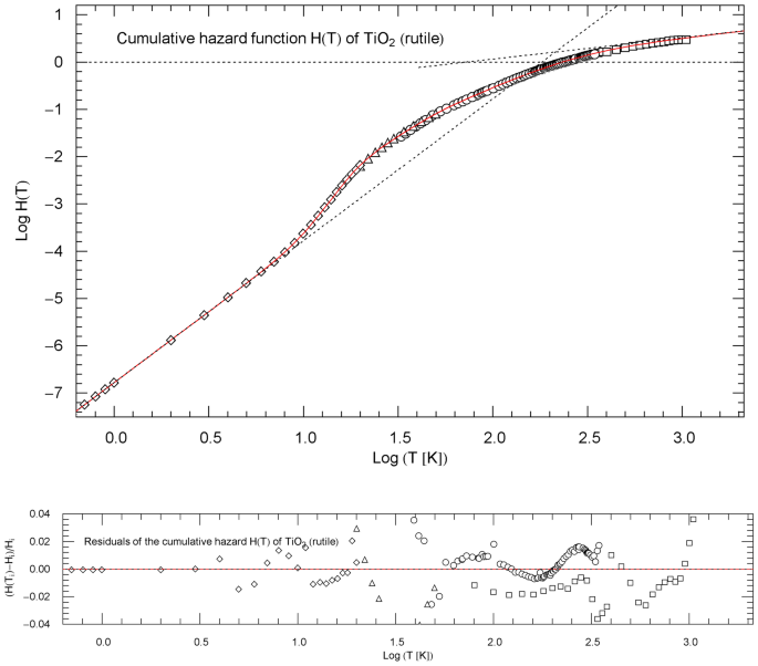
Cumulative hazard function (CHF) $H(T)$ of rutile (titanium dioxide), cf. Sect. 4.1. The data points are based on isochoric heat-capacity data of Ref. [18] (squares), Ref. [19] (circles), Ref. [20] (triangles) and Ref. [21] (diamonds). The conversion of the heat-capacity data to data points of the CHF is explained in Sect. 2. The red solid curve depicts the multiply broken power-law density $H(T)$ in (7), with regressed parameters in Table 1. The least-squares functional (5) was used for regression. The asymptotic low- and high-temperature power-law limits of $H(T)$, cf. Sect. 3, are indicated as black dotted straight lines; their amplitudes and exponents are listed in Table 1. The depicted temperature range terminates at the melting point of 2113 K. Residual relative deviations of the regressed CHF from the data points are shown in the lower panel

Fig. 2

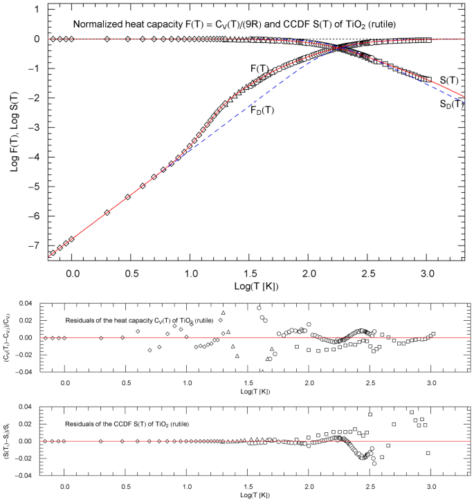
Normalized heat capacity $F(T) = C_{V} (T)/(9R)$ of rutile, and complementary cumulative distribution (CCDF) $S(T) = 1 - F(T) = \exp ( - H(T))$, cf. Sect. 4.1. The depicted normalized heat-capacity data stem from Ref. [18] (squares), Ref. [19] (circles), Ref. [20] (triangles) and Ref. [21] (diamonds). The data points of the CCDF $S(T)$ are obtained from the heat-capacity data, cf. Sect. 2. $F(T)$ and $S(T)$ (red solid curves) are calculated from the regressed cumulative hazard function $H(T)$ in Fig. 1. The temperature range is cut off at the melting point. The blue dashed curves indicate the normalized Debye heat capacity $F_{{\text{D}}} (T) = C_{{\text{D}}} (T)/(9R)$ and the associated CCDF $S_{{\text{D}}} (T) = 1 - F_{{\text{D}}} (T)$ calculated via (8) with $\theta = 777.8{\text{ K}}$. The lower panels show the residuals of the regressed heat capacity $C_{V} (T)$ and CCDF $S(T)$

Fig. 3

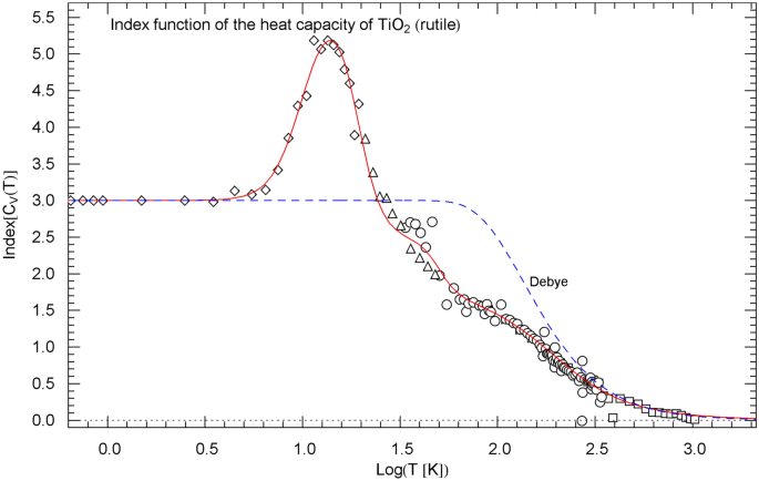
Index function ${\text{Index[}}C_{V} (T)]$ of the regressed heat capacity of rutile, cf. Sect. 5. The depicted data points are obtained as finite differences from the heat-capacity data of Ref. [18] (squares), Ref. [19] (circles), Ref. [20] (triangles) and Ref. [21] (diamonds), cf. (14). The red solid Index curve represents the Log–Log slope of the regressed heat capacity $C_{V}(T)$ (depicted in Fig. 2 in Log–Log coordinates) and is calculated as indicated in (11)–(13), with regressed parameters in Table 1. The blue dashed curve shows the Index function ${\text{Index[}}C_{{\text{D}}} (T)]$ of the Debye heat capacity (see Fig. 2), calculated as stated in (17) with $\theta = 777.8{\text{ K}}$

Fig. 4

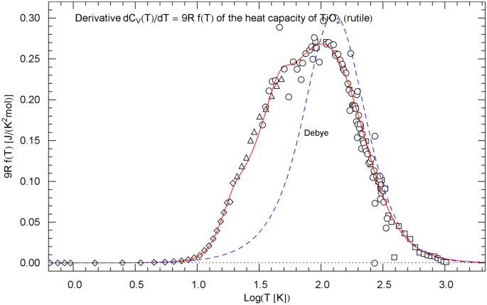
Temperature derivative $C^{\prime}_{V} (T)$ of the isochoric heat capacity of rutile, cf. Sect. 5. The data points are obtained as finite differences from the heat-capacity data of Ref. [18] (squares), Ref. [19] (circles), Ref. [20] (triangles) and Ref. [21] (diamonds), see after (15). $C^{\prime}_{V} (T) = 9Rf(T)$ is depicted as red solid curve. The probability density $f(T)$ in (15) is assembled from the regressed cumulative hazard function $H(T)$ in Fig. 1 and its Index function ${\text{Index[}}H(T)]$ in (13), with parameters in Table 1. The derivative of the Debye heat capacity $C^{\prime}_{{\text{D}}} (T)$ is shown as blue dashed curve, calculated via (16) with $\theta = 777.8{\text{ K}}$

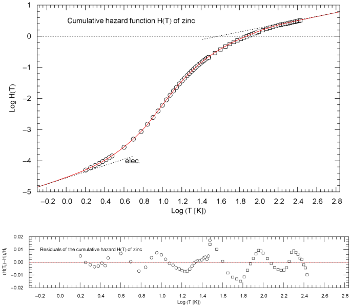
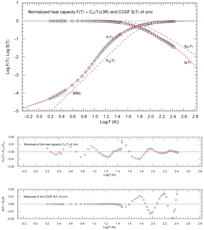
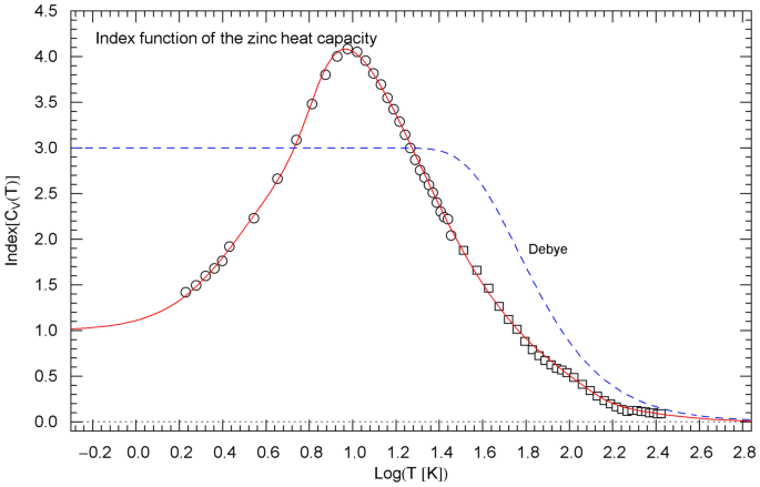
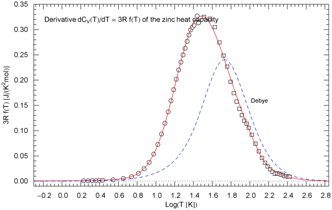
In Sect. 4.2, the heat capacity of zinc is calculated from the regressed CHF, cf. Figs. 5, 6, 7, 8, based on data tables from Refs. [22,23,24]. In contrast to the non-conducting ${\text{TiO}}_{{2}}$ compound, the cubic low-temperature slope generated by atomic vibrations is overpowered by the linear low-temperature scaling of the heat capacity of the conduction electrons. The regressed heat capacity is compared with the Debye model, using the Debye temperature of zinc quoted in Ref. [25].

Fig. 5

Cumulative hazard function (CHF) $H(T)$ of zinc, cf. Sect. 4.2. The data points are based on isochoric heat-capacity data of Refs. [22, 23] (circles) and Ref. [24] (squares). The conversion of the heat-capacity data to data points of the CHF is explained in Sect. 2. The red solid curve is a plot of the multiply broken power-law density $H(T)$ in (9), with regressed parameters in Table 1. The asymptotic low- and high-temperature power-law limits of $H(T)$, cf. Sect. 3, are depicted as black dotted straight lines, with amplitudes and exponents listed in Table 1. The low-temperature asymptote shows the linear electronic power law. The temperature range of the figure terminates at the zinc melting point of 693 K. Residual relative deviations of the regressed CHF from the data points are depicted in the lower panel

Fig. 6

Normalized heat capacity $F(T) = C_{V} (T)/(3R)$ of zinc, and complementary cumulative distribution (CCDF) $S(T) = 1 - F(T) = \exp ( - H(T))$, cf. Sect. 4.2. The depicted heat-capacity data (normalized) are tabulated in Refs. [22, 23] (circles) and Ref. [24] (squares). The data points of the CCDF $S(T)$ are obtained from the heat-capacity data as outlined in Sect. 2. $F(T)$ and $S(T)$ (red solid curves) are calculated from the regressed cumulative hazard function $H(T)$ in Fig. 5. The black dotted low-temperature asymptote indicates the linear electronic power-law scaling. The temperature range is cut off at the melting point. The blue dashed curves show the normalized Debye heat capacity $F_{{\text{D}}} (T) = C_{{\text{D}}} (T)/(3R)$ and the associated CCDF $S_{{\text{D}}} (T) = 1 - F_{{\text{D}}} (T)$ calculated from (8) with $\theta = 329{\text{ K}}$. The lower panels depict the residuals of the regressed heat capacity $C_{V} (T)$ and CCDF $S(T)$

Fig. 7

Index function ${\text{Index[}}C_{V} (T)]$ of the regressed heat capacity of zinc, cf. Sect. 5. The depicted data points are obtained as finite differences from the heat-capacity data of Refs. [22, 23] (circles) and Ref. [24] (squares), cf. (14). The red solid Index curve represents the Log–Log slope of the regressed heat capacity $C_{V}(T)$ (depicted in Fig. 6 in Log–Log coordinates) and is calculated as indicated in (11)–(13) with regressed parameters in Table 1. The blue dashed curve shows the Index function ${\text{Index[}}C_{{\text{D}}} (T)]$ of the Debye heat capacity (Fig. 6), calculated as stated in (17) with $\theta = 329{\text{ K}}$

Fig. 8

Temperature derivative $C^{\prime}_{V} (T)$ of the isochoric heat capacity of zinc, cf. Sect. 5. The data points are obtained as finite differences from the heat-capacity data of Refs. [22, 23] (circles) and Ref. [24] (squares), see after (15). $C^{\prime}_{V} (T) = 3Rf(T)$ is depicted as red solid curve. The probability density $f(T)$ in (15) is assembled from the regressed cumulative hazard function $H(T)$ in Fig. 5 and its Index function ${\text{Index[}}H(T)]$ in (13), with parameters in Table 1. The derivative of the Debye heat capacity $C^{\prime}_{{\text{D}}} (T)$ is shown as blue dashed curve, calculated via (16) with $\theta = 329{\text{ K}}$

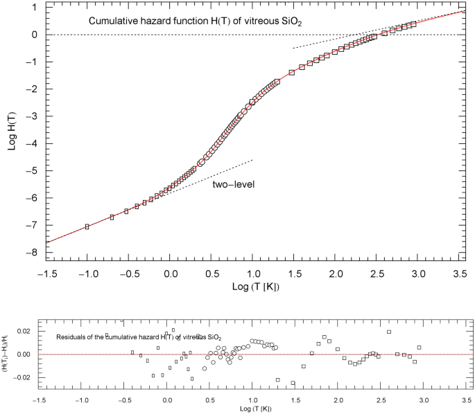
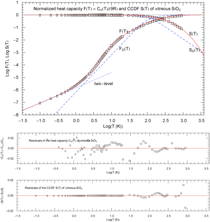
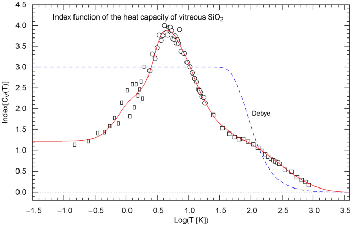
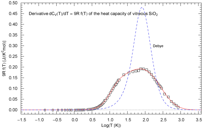
In Sect. 4.3, the CHF and heat capacity of vitreous silica is studied, cf. Figs. 9, 10, 11, 12. In contrast to the crystals considered in Sects. 4.1 and 4.2, the low-temperature slope of the CHF and heat capacity of this glass is a non-integer power law, slightly nonlinear and generated by a two-level Fermi system [26, 27]. Heat-capacity data of Refs. [28,29,30] are used to regress the CHF of ${\text{v - SiO}}_{{2}}$.

Fig. 9

Cumulative hazard function (CHF) $H(T)$ of vitreous silica, cf. Sect. 4.3. The data points are based on isochoric heat-capacity data of Ref. [28] (rectangles), Ref. [29] (circles) and Ref. [30] (squares). The conversion of the heat-capacity data to data points of the CHF is explained in Sect. 2. The red solid curve depicts the multiply broken power-law density $H(T)$ in (10), with regressed parameters in Table 1. The asymptotic low- and high-temperature power-law limits of $H(T)$, cf. Sect. 3, are indicated as black dotted straight lines; their amplitudes and exponents are listed in Table 1. The asymptotic low-temperature slope is generated by a fermionic two-level system. The temperature range terminates at the melting point of 1986 K. Residual relative deviations of the regressed CHF from the data points are shown in the lower panel

Fig. 10

Normalized heat capacity $F(T) = C_{V} (T)/(9R)$ of ${\text{v - SiO}}_{{2}}$, and complementary cumulative distribution (CCDF) $S(T) = 1 - F(T) = \exp ( - H(T))$, cf. Sect. 4.3. The depicted normalized heat-capacity data stem from Ref. [28] (rectangles), Ref. [29] (circles) and Ref. [30] (squares). The data points of the CCDF $S(T)$ are obtained from the heat-capacity data, cf. Sect. 2. $F(T)$ and $S(T)$ (red solid curves) are calculated from the regressed cumulative hazard function $H(T)$ in Fig. 9. The blue dotted low-temperature asymptote indicates the power-law scaling of the two-level Fermi system. The temperature range is cut off at the melting point. The blue dashed curves show the normalized Debye heat capacity $F_{{\text{D}}} (T) = C_{{\text{D}}} (T)/(9R)$ and the associated CCDF $S_{{\text{D}}} (T) = 1 - F_{{\text{D}}} (T)$ calculated via (8) with $\theta = 495{\text{ K}}$. The lower panels depict the residuals of the regressed heat capacity $C_{V} (T)$ and CCDF $S(T)$

Fig. 11

Index function ${\text{Index[}}C_{V} (T)]$ of the regressed heat capacity of ${\text{v - SiO}}_{{2}}$, cf. Sect. 5. The depicted data points are obtained as finite differences from the heat-capacity data of Ref. [28] (rectangles), Ref. [29] (circles) and Ref. [30] (squares), cf. (14). The red solid Index curve represents the Log–Log slope of the regressed heat capacity $C_{V}(T)$ (depicted in Fig. 10 in Log–Log coordinates) and is calculated as indicated in (11)–(13) with regressed parameters in Table 1. The blue dashed curve shows the Index function ${\text{Index[}}C_{{\text{D}}} (T)]$ of the Debye heat capacity (Fig. 10), calculated as stated in (17) with $\theta = 495{\text{ K}}$

Fig. 12

Temperature derivative $C^{\prime}_{V} (T)$ of the isochoric heat capacity of ${\text{v - SiO}}_{{2}}$, cf. Sect. 5. The data points are obtained as finite differences from the heat-capacity data of Ref. [28] (rectangles), Ref. [29] (circles) and Ref. [30] (squares), see after (15). $C^{\prime}_{V} (T) = 9Rf(T)$ is depicted as red solid curve. The probability density $f(T)$ in (15) is assembled from the regressed cumulative hazard function $H(T)$ in Fig. 9 and its Index function ${\text{Index[}}H(T)]$ in (13), with parameters in Table 1. The derivative of the Debye heat capacity $C^{\prime}_{{\text{D}}} (T)$ is shown as blue dashed curve, calculated via (16) with $\theta = 495{\text{ K}}$

In Sect. 5, we compare the Log–Log slope of the regressed heat capacity with the Debye theory. This is done by calculating the Index function representing the local power-law exponent of the heat capacity, see Figs. 3, 7, 11. In Log–Log coordinates used for the plots of the heat capacities, the Index is just the slope of the tangent line to the heat-capacity curve at the respective temperature. The data points of the Index function are extracted from the heat-capacity data by way of finite-difference methods. Also in Sect. 5, we discuss the underlying empirical probability density $f(T)$, cf. Ref. [31], which is, up to a normalization constant, the temperature derivative of the regressed heat capacity. The data points for $f(T)$ are obtained as finite differences from the data sets of the heat capacity, see Figs. 4, 8, 12.

In Sect. 6, the equilibrium entropy and internal energy obtained from the regressed isochoric heat capacities is studied. Integral representations of these functions are derived as expectation values over the probability density $f(T)$. We also calculate the low- and high-temperature asymptotics of entropy and internal energy, in particular the next-to-leading orders of the high-temperature expansions, and compare with the respective limits of the Debye model. Section 7 summarizes the conclusions.

2 Relating isochoric heat capacities to hazard functions

The use of cumulative hazard functions in the modeling of isochoric heat capacities $C_{V} (T)$ of solids is based on the fact that $C_{V} (T)$ is an increasing continuous function (leaving aside polymorphic transitions, melting, sublimation, etc.) starting from zero at $T = 0$ and reaching a constant plateau value in the classical high-temperature limit $C_{V} (T)\sim 3n_{{\text{a/f}}} R$. Here, $n_{{\text{a/f}}}$ denotes the number of atoms per formula unit and $R = 8.3145{\text{ J/(K mol)}}$ is the gas constant; molar units will be used. The normalized heat capacity $F(T) = C_{V} (T)/(3n_{{\text{a/f}}} R)$ is thus the cumulative distribution function (CDF) of a probability density (pdf) $f(T) = F^{\prime}(T)$.

The complementary cumulative distribution (CCDF) $S(T) = 1 - F(T)$ is decreasing from one at $T = 0$ to zero in the high-temperature limit. The cumulative hazard function is defined as $H(T) = - \log S(T)$, which is an increasing function from zero at $T = 0$ to infinity in the high-temperature limit. Thus, $S(T) = \exp ( - H(T))$, and the normalized heat capacity can be represented as $F(T) = 1 - \exp ( - H(T))$. In the low-temperature regime, $F(T)$ and $H(T)$ coincide asymptotically, $F(T)\sim H(T)$. We will use the cumulative hazard function $H(T)$ as the primary function, regressing it from heat-capacity data. All other functions enumerated above can be calculated from the regressed $H(T)$.

In particular, the pdf is found as $f(T) = h(T)\exp ( - H(T))$, where $h(T) = H^{\prime}(T)$ is the differential hazard rate. We will assume that the regressed $H(T)$ has power-law asymptotics both in the low- and high-temperature regime, $H(T \to 0)\sim a_{0} T^{{\alpha_{0} }}$ and $H(T \to \infty )\sim a_{\infty } T^{{\alpha_{\infty } }}$, with positive powers $\alpha_{0}$ and $\alpha_{\infty }$. This ensures that $f(T)$ is integrable and normalized to one, since $F(T) = \int_{0}^{T} {f(T){\text{d}}T}$, and that all moments are finite, since $f(T)$ is exponentially decaying, admitting stretched, compressed or regular exponential decay, depending on whether $0 < \alpha_{\infty } < 1$, $\alpha_{\infty } > 1$, or $\alpha_{\infty } = 1$, respectively. As for the low-temperature power-law index $\alpha_{0}$, we will study three examples: rutile, where the low-temperature index $\alpha_{0} = 3$ is generated by lattice vibrations, zinc, where the exponent $\alpha_{0} = 1$ is generated by an electron gas overpowering the low-temperature heat capacity of atomic vibrations, and vitreous ${\text{SiO}}_{{2}}$, where the non-integer index $\alpha_{0} \approx 1.22$ is due to a fermionic two-level system.

The data points of the molar isochoric heat capacity $C_{{\text{V}}} (T)$ will be denoted by $(T_{i} [{\text{K}}],C_{V,i} [{\text{J/(K mol)}}])_{i = 1,\ldots,N}$, with units as indicated. Data points of the normalized heat capacity $F(T)$ are labeled $(T_{i} [{\text{K}}],F_{i} )_{i = 1,\ldots,N}$, with $F_{i} = C_{V,i} /(3n_{{\text{a/f}}} R)$. Data points of the CCDF $S(T)$ are denoted by $(T_{i} [{\text{K}}],S_{i} )_{i = 1,\ldots,N}$, $S_{i} = 1 - F_{i}$, and data points for the cumulative hazard function $H(T)$ are labeled $(T_{i} [{\text{K}}],H_{i} )_{i = 1,\ldots,N}$, $H_{i} = - \log S_{i}$. We will model empirical heat capacities from zero temperature up to the melting point where $C_{V} (T)$ has a discontinuity indicating a first-order transition.

3 Cumulative hazard functions as multiply broken power-law densities

We will employ a multiply broken power-law density as cumulative hazard function, cf., e.g., Ref. [32],

$$H(T) = a_{0} T^{{\alpha_{0} }} \prod\limits_{k = 0}^{n} {(1 + b_{k} T^{{\beta_{k} }} )^{{\eta_{k} }} },$$

(1)

where $a_{0}$, $b_{k}$ are positive amplitudes, $\alpha_{0}$ and $\beta_{k}$ are positive exponents and the $\eta_{k}$ are real non-zero exponents to be inferred by least-squares regression. The number of factors in the product is adapted to the data set. The asymptotic limits of $H(T)$ in (1) are simple power laws, $H(T \to 0)\sim a_{0} T^{{\alpha_{0} }}$ and $H(T \to \infty )\sim a_{\infty } T^{{\alpha_{\infty } }}$, with $\alpha_{\infty } : = \alpha_{0} + \sum\nolimits_{k = 0}^{n} {\beta_{k} \eta_{k} }$ and $a_{\infty } : = a_{0} \prod\nolimits_{k = 0}^{n} {b_{k}^{{\eta_{k} }} }$. The representation (1) is suitable for low-temperature expansions. To obtain high-temperature ascending series expansions in $1/T$, we rewrite $H(T)$ in (1) as

$$H(T) = a_{\infty } T^{{\alpha_{\infty } }} \prod\limits_{k = 0}^{n} {(1 + 1/(b_{k} T^{{\beta_{k} }} ))^{{ \, \eta_{k} }} }.$$

(2)

Each of the factors in (1) and (2) admits an ascending series expansion in integer powers of $T^{{\beta_{k} }}$ or $1/T^{{\beta_{k} }}$,  which is absolutely convergent within $T < b_{k}^{{ - 1/\beta_{k} }}$ or $T > b_{k}^{{ - 1/\beta_{k} }}$, respectively. Multiplication of the power-series expansions of the factors in the product (1) or (2) and reordering the series in ascending real powers of $T$ or $1/T$ gives a Hahn series, which is absolutely convergent in the smallest convergence domain of the expanded factors, that is $T < \min (b_{k}^{{ - 1/\beta_{k} }} )_{k = 1,\ldots,n}$ or $T > \max (b_{k}^{{ - 1/\beta_{k} }} )_{k = 1,\ldots,n}$, respectively.

Specifically,

$$H(T \to 0)\sim H_{0} (T) = a_{0} T^{{\alpha_{0} }} (1 + \eta_{m} b_{m} T^{{\beta_{m} }} + \cdots ),$$

(3)

$$H(T \to \infty )\sim H_{\infty } (T) = a_{\infty } T^{{\alpha_{\infty } }} (1 + \frac{{\eta_{m} }}{{b_{m} T^{{\beta_{m} }} }} + \cdots ),$$

(4)

where $\beta_{m}$ is the smallest of the exponents $\beta_{k}$. Higher orders of these series can be calculated as outlined above, once the exponents $\beta_{k}$ are specified numerically. The non-integer exponents of the series expansions (3) and (4) constitute an unbounded increasing sequence of real numbers.

The least-squares regression is performed with $H(T)$ in (1), and the nonlinear least-squares functional reads

$$\chi_{H}^{2} (a_{0} ,\alpha_{0} ,(b_{k}^{{}} ,\beta_{k}^{{}} ,\eta_{k}^{{}} )_{k = 0,\ldots,n} ) = \sum\limits_{i = 1}^{N} {\frac{{(H(T_{i} ) - H_{i} )^{2} }}{{H_{i}^{2} }}},$$

(5)

with data points $(T_{i} ,H_{i} )_{i = 1,\ldots,N}$ as in Sect. 2. $H(T)$ depends on the fitting parameters $a_{0} ,\alpha_{0} ,(b_{k}^{{}} ,\beta_{k}^{{}} ,\eta_{k}^{{}} )_{k = 0,\ldots,n}$.

To find initial values for the parameters when minimizing the least-squares functional, it is convenient to reparametrize $H(T)$ in (1) as

$$H(T) = a_{0} T^{{\alpha _{0} }} \prod\limits_{{k = 0}}^{n} {(1 + (T/10^{{\hat{b}_{k} }} )^{{\hat{\beta }_{k} /\left| {\hat{\eta }_{k} } \right|}} )^{{\hat{\eta }_{k} }} } ,$$

(6)

where $\hat{b}_{k} = {\text{Log}}(b_{k}^{{ - 1/\beta_{k} }} )$, $\hat{\beta }_{k} = \beta_{k} \left| {\eta_{k} } \right|$, $\hat{\eta }_{k} = \eta_{k}$, and to plot the data set in decadic Log–Log coordinates as done in the figures, since simple power laws such as the asymptotic limits of $H(T)$ appear as straight lines in this representation. The parameters in (1) are recovered as $b_{k} = (10^{{ - \hat{b}_{k} }} )^{{\hat{\beta }_{k} /\left| {\hat{\eta }_{k} } \right|}}$, $\beta_{k} = \hat{\beta }_{k} /\left| {\hat{\eta }_{k} } \right|$, $\eta_{k} = \hat{\eta }_{k}$. A method to systematically find initial parameter values for the nonlinear least-squares regression of factorizing multiparameter densities is outlined in Refs. [31,32]. In Sect. 4, a Mathematica^® [33] routine, FindMinimum[chisquared[…],{initial values}, MaxIterations → nmax], will be used for the iteration of the multiparametric least-squares functional (5).

4 Isochoric heat capacities of specific materials: regression of the cumulative hazard function

4.1 Rutile polymorph of titanium dioxide

The data sets of the rutile (${\text{TiO}}_{{2}}$) heat capacity, cf. Refs. [18,19,20,21], are converted to a data set $(T_{i} ,H_{i} )_{i = 1,\ldots,N}$ of the cumulative hazard function (CHF) $H(T)$ as explained in Sect. 2, which is depicted in Fig. 1. The CHF is specified as broken power-law density (see (1))

$$H(T) = a_{0} T^{3} (1 + b_{0} T^{{\beta_{0} }} )^{{\eta_{0} }} \frac{1}{{(1 + b_{1} T^{{\beta_{1} }} )^{{\eta_{1} }} }}\frac{1}{{(1 + b_{2} T^{{\beta_{2} }} )^{{\eta_{2} }} }}\frac{1}{{(1 + b_{3} T^{{\beta_{3} }} )^{{\eta_{3} }} }},$$

(7)

with positive amplitudes $a_{0}$ and $b_{k}$ and positive exponents $\beta_{k}$ and $\eta_{k}$. The exponent $\alpha_{0}$ in (1) is fixed from the outset as $\alpha_{0} = 3$, to recover the cubic low-temperature scaling, since $C_{V} (T)/(3n_{{\text{a/f}}} R) = F(T)\sim H(T)$, with $n_{{\text{a/f}}} = 3$, cf. Sect. 2. The regression is performed with the least-squares functional (5). The regressed parameters and the goodness-of-fit parameters are listed in Table 1, including the amplitude and exponent of the high-temperature power-law limit $H(T)\sim a_{\infty } T^{{\alpha_{\infty } }}$.

Table 1 Fitting parameters of the cumulative hazard function (CHF) $H(T)$ of rutile, zinc and ${\text{v - SiO}}_{{2}}$

Figure 2 depicts the regressed normalized heat capacity $F(T) = 1 - \exp ( - H(T))$ and the CCDF $S(T) = \exp ( - H(T))$, as well as the respective data sets $(T_{i} ,F_{i} )_{i = 1,\ldots,N}$ and $(T_{i} ,S_{i} )_{i = 1,\ldots,N}$, cf. Sect. 2. Residual panels are also included in Figs. 1 and 2, indicating the local accuracy of the regressed functions. The temperature range of the figures extends to the melting point of 2113 K.

Figure 2 also shows the Debye approximations of the normalized heat capacity $F(T)$ and the CCDF $S(T)$, with Debye temperature $\theta = 777.8{\text{ K}}$ calculated from the regressed amplitude $a_{0}$ in (7) and Table 1, $\theta = (4\pi^{4} /(5a_{0} ))^{1/3}$. The Debye heat capacity $C_{{\text{D}}} (T)$ and the normalized version $F_{{\text{D}}} (T)$ thereof (which is plotted in Fig. 2) read

$$\frac{{C_{{\text{D}}} (T)}}{{3n_{{\text{a/f}}} R}} = F_{{\text{D}}} (T) = 12D(d) - \frac{3d}{{{\text{e}}^{d} - 1}},\;D(d): = \frac{1}{{d_{{}}^{3} }}\int\limits_{0}^{d} {\frac{{y^{3} {\text{d}}y}}{{{\text{e}}^{y} - 1}}} ,$$

(8)

with $d = \theta /T$. Also indicated in Fig. 2 is the CCDF of the Debye theory, $S_{{\text{D}}} (T) = 1 - F_{{\text{D}}} (T)$. Evidently, the Debye model reproduces the classical limit and the cubic low-temperature scaling, but is otherwise not accurate in the crossover region, substantially underestimating the heat capacity data. For future reference, we also define, in analogy to Sect. 2, the cumulative hazard function and hazard rate of the Debye model as $H_{{\text{D}}} (T) = - \log S_{{\text{D}}} (T)$ and $h_{{\text{D}}} (T) = H^{\prime}_{{\text{D}}} (T)$ as well as the probability density $f_{{\text{D}}} (T) = F^{\prime}_{{\text{D}}} (T)$ (explicitly stated in (16)) and also note $h_{{\text{D}}} (T) = f_{{\text{D}}} (T)/S_{{\text{D}}} (T)$.

4.2 Zinc

The heat-capacity data of zinc, taken from tables in Refs. [22,23,24], are converted to the data set $(T_{i} ,H_{i} )_{i = 1,\ldots,N}$ of the CHF $H(T)$ depicted in Fig. 5. For the least-squares fit, we use the multiply broken power law (cf. (1))

$$H(T) = a_{0} T(1 + b_{0} T^{{\beta_{0} }} )^{{\eta_{0} }} (1 + b_{1} T^{{\beta_{1} }} )^{{\eta_{1} }} \frac{1}{{(1 + b_{2} T^{{\beta_{2} }} )^{{\eta_{2} }} }}\frac{1}{{(1 + b_{3} T^{{\beta_{3} }} )^{{\eta_{3} }} }},$$

(9)

depending on positive parameters $a_{0}$,$b_{k}$,$\beta_{k}$,$\eta_{k}$. The low-temperature limit of $H(T)$ and of the normalized heat capacity coincide, $C_{V} (T)/(3n_{{\text{a/f}}} R) = F(T)\sim H(T)$, with $n_{{\text{a/f}}} = 1$, see also Sect. 6. We have identified $\alpha_{0} = 1$ as low-temperature exponent in (9) to account for the linear electronic power-law limit of the heat capacity. The least-squares functional used for regression is stated in (5), and the regressed parameters of $H(T)$ are listed in Table 1.

Figure 6 depicts the regressed normalized heat capacity $F(T) = 1 - \exp ( - H(T))$ and the CCDF $S(T) = \exp ( - H(T))$ of zinc and the corresponding data sets $(T_{i} ,F_{i} )_{i = 1,\ldots,N}$ and $(T_{i} ,S_{i} )_{i = 1,\ldots,N}$. The temperature range in Figs. 5 and 6 is cut off at the melting point of 693 K. For comparison, we have also indicated, in Fig. 6, the counterparts to $F(T)$ and $S(T)$ in the Debye model, that is $F_{{\text{D}}} (T)$ and $S_{{\text{D}}} (T)$ as defined in (8), with Debye temperature of 329 K, cf. Ref. [25].

4.3 Vitreous ${\text{SiO}}_{{2}}$

The heat-capacity data of ${\text{v - SiO}}_{{2}}$ from Refs. [28,29,30] are converted to data points $(T_{i} ,H_{i} )_{i = 1,\ldots,N}$ of the CHF $H(T)$, cf. Sect. 2, and are plotted in Fig. 9. The least-squares fit to the $(T_{i} ,H_{i} )_{i = 1,\ldots,N}$ data is performed with the multiply broken power law (cf. (1))

$$H(T) = a_{0} T^{{\alpha_{0} }} (1 + b_{0} T^{{\beta_{0} }} )^{{\eta_{0} }} (1 + b_{1} T^{{\beta_{1} }} )^{{\eta_{1} }} \frac{1}{{(1 + b_{2} T^{{\beta_{2} }} )^{{\eta_{2} }} }}\frac{1}{{(1 + b_{3} T^{{\beta_{3} }} )^{{\eta_{3} }} }} ,$$

(10)

with positive parameters $a_{0}$,$b_{k}$,$\beta_{k}$,$\eta_{k}$. The low-temperature slope $H(T)\sim a_{0} T^{{\alpha_{0} }}$ coincides with the low-temperature limit of the normalized molar heat capacity $F(T)$. The empirical exponent $\alpha_{0} = 1.22$ originating from a fermionic two-level system, cf. Refs. [26, 27], is taken as fixed input in the regression. The regressed parameters and goodness-of-fit parameters are listed in Table 1. The normalized heat capacity $F(T) = 1 - \exp ( - H(T))$ of ${\text{v - SiO}}_{{2}}$ and the CCDF are depicted in Fig. 10, including the respective data points $(T_{i} ,F_{i} )_{i = 1,\ldots,N}$ and $(T_{i} ,S_{i} )_{i = 1,\ldots,N}$. Residual panels of the regressed functions are included in Figs. 9 and 10. The depicted temperature range in these figures extends to 1986 K, the melting point of ${\text{v - SiO}}_{{2}}$. The normalized heat capacity $F_{{\text{D}}} (T)$ and CCFD $S_{{\text{D}}} (T)$ of the Debye model are also indicated in Fig. 10 for comparison, calculated as stated in (8) with Debye temperature of 495 K inferred from elastic constants, cf. Ref. [29].

5 Index functions and probability density

The Index functional of a positive function $F(T)$ on the positive real axis is defined as, cf., e.g., Ref. [12],

$${\text{Index[}}F(T)] = \frac{{{\text{d}}\log F(T)}}{{{\text{d}}\log T}} = T\frac{{F^{\prime}(T)}}{F(T)}.$$

(11)

${\text{Index[}}F(T)]$ gives the local slope of $F(T)$ when plotted in Log–Log coordinates, as done in Figs. 2, 6 and 10 depicting the normalized heat capacity $F(T) = C_{V} (T)/(3n_{{\text{a/f}}} R)$. Evidently, ${\text{Index[}}C_{V} (T)] = {\text{Index[}}F(T)]$.

The Index of the cumulative hazard functions (CHFs) in Figs. 1, 5, 9 reads ${\text{Index[}}H(T)] = TH^{\prime}(T)/H(T)$. The Index functions of the normalized heat capacity $F(T)$ and CHF $H(T)$ are related by the identity

$${\text{Index[}}F(T)] = \frac{H(T)}{{\exp (H(T)) - 1}}{\text{Index[}}H(T)].$$

(12)

Specifying the CHF $H(T)$ as multiply broken power-law density (1), we find

$${\text{Index[}}H(T)] = \alpha_{0} + \sum\limits_{k = 0}^{n} {\beta_{k} \eta_{k} \frac{{b_{k} T^{{\beta_{k} }} }}{{1 + b_{k} T^{{\beta_{k} }} }}} .$$

(13)

The Index function of the normalized heat capacity $F(T)$ can thus be calculated by way of (12), with $H(T)$ in (1) and ${\text{Index[}}H(T)]$ in (13). Also, ${\text{Index[}}H(T \to 0)] = \alpha_{0}$ and ${\text{Index[}}H(T \to \infty )] = \alpha_{\infty }$, cf. Sect. 3.

The data points of the Index function ${\text{Index[}}F(T)]$ can be assembled from the $(T_{i} ,F_{i} )_{i = 1,\ldots,N}$ data (of the normalized heat capacity, cf. Sect. 2) as $((T_{j} + T_{j + 1} )/2,{\text{Index[}}F]_{j} )_{j = 1,\ldots,N - 1}$, where

$${\text{Index[}}F]_{j} = \frac{{\log (F_{j + 1} /F_{j} )}}{{\log (T_{j + 1} /T_{j} )}}$$

(14)

is the finite-difference version of the derivative ${\text{d}}\log F(T)/{\text{d}}\log T$ in (11), see Figs. 3, 7, 11.

The probability density $f(T) = F^{\prime}(T)$ can also be calculated from (1) and (13), by way of the identity

$$f(T) = \exp ( - H(T))\frac{H(T)}{T}{\text{Index[}}H(T)].$$

(15)

The data points of $f(T)$ are assembled from the $(T_{i} ,F_{i} )_{i = 1,\ldots,N}$ data as finite differences $((T_{j} + T_{j + 1} )/2,f_{j} )_{j = 1,\ldots,N - 1}$, with $f_{j} = (F_{j + 1} - F_{j} )/(T_{j + 1} - T_{j} )$. The derivative of the isochoric heat capacity is proportional to the probability density, $C^{\prime}_{V} (T) = 3n_{{\text{a/f}}} Rf(T)$, and the data points of $C^{\prime}_{V} (T)$ are obtained as $((T_{j} + T_{j + 1} )/2, \, 3n_{{\text{a/f}}} Rf_{j} )_{j = 1,\ldots,N - 1}$, see Figs. 4, 8 and 12.

As for the Debye theory, the normalized heat capacity $F_{{\text{D}}} (T) = C_{{\text{D}}} (T)/(3n_{{\text{a/f}}} R)$ is stated in (8), and its temperature derivative, the probability density $f_{{\text{D}}} (T) = F^{\prime}_{{\text{D}}} (T)$, cf. Sect. 2, reads

$$f_{{\text{D}}} (T) = \frac{3}{T}(F_{{\text{D}}} (T) - \frac{{d^{2} {\text{e}}^{d} }}{{{\text{(e}}^{d} - 1)^{2} }})$$

(16)

with $d = \theta /T$. The derivative of the Debye heat capacity is $C^{\prime}_{{\text{D}}} (T) = 3n_{{\text{a/f}}} Rf_{{\text{D}}} (T)$, which is plotted in Figs. 4, 8, 12 for comparison with the derivative of the regressed empirical heat capacity $C^{\prime}_{V} (T) = 3n_{{\text{a/f}}} Rf(T)$.

The Index function of the normalized Debye heat capacity $F_{{\text{D}}} (T)$ representing the local Log–Log slope of $C_{{\text{D}}} (T)$ and $F_{{\text{D}}} (T)$ reads

$${\text{Index[}}F_{{\text{D}}} (T)] = T\frac{{F^{\prime}_{{\text{D}}} (T)}}{{F_{{\text{D}}} (T)}} = 3(1 - \frac{1}{{F_{{\text{D}}} (T)}}\frac{{d^{2} {\text{e}}^{d} }}{{{\text{(e}}^{d} - 1)^{2} }}),$$

(17)

with $F_{{\text{D}}} (T)$ in (8) substituted. The normalization does not affect the Log–Log slope, which is depicted in Figs. 3, 7, 11 for comparison with the empirical Index function ${\text{Index[}}C_{V} (T)]$ of rutile, zinc and ${\text{v - SiO}}_{{2}}$.

6 Integral representations and asymptotic expansions of entropy and internal energy

Entropy $S_{{\text{E}}} = 3n_{{\text{a/f}}} Rs(T)$ and internal energy $U_{{\text{E}}} = 3n_{{\text{a/f}}} Ru(T)$ are defined by the normalized functions

$$s(T) = \int\limits_{0}^{T} {\frac{1}{t}F(t)} {\text{d}}t,\;u(T) = \int\limits_{0}^{T} {F(t)} {\text{d}}t,$$

(18)

where $F(T) = C_{V} (T)/(3n_{{\text{a/f}}} R)$ is the normalized molar isochoric heat capacity, $n_{{\text{a/f}}}$ the number of atoms per formula unit, and $R$ the gas constant, cf. Sect. 2. These integral representations ensure that the equilibrium condition ${\text{d}}s(T(u))/{\text{d}}u = 1/T$ is satisfied, where $T(u)$ is the inverse of $u(T)$ in (18). Entropy and internal energy are only defined up to an additive constant, which is chosen so that these quantities vanish at zero temperature, $s(0) = 0$ and $u(0) = 0$.

Both $s(T)$ and $u(T)$ can be written as expectation values over the probability density $f(T)$, cf. Sect. 2,

$$u(T) = \int\limits_{0}^{\infty } {(T - t)\Theta (T - t)f(t){\text{d}}t} ,\;s(T) = \int\limits_{0}^{\infty } {\log (T/t)\Theta (T - t)f(t){\text{d}}t},$$

(19)

where $\Theta (t)$ is the Heaviside step function. The equivalence of representations (18) and (19) can be seen by differentiation, the derivative of the Heaviside function being the Dirac delta function, $\Theta^{\prime}(t) = \delta (t)$.

For comparison, the Debye model, cf. Sect. 4.1, gives the normalized internal energy $u_{{\text{D}}} (T) = 3TD(d)$ (where the zero-point energy has been dropped) and entropy $s_{{\text{D}}} (T) = 4D(d) - \log (1 - {\text{e}}^{ - d} )$ (also vanishing at $T = 0$). The Debye function $D(d)$ is defined in (8), with $d = \theta /T$ and Debye temperature $\theta$.

In the following, we compare the low- and high-temperature asymptotics of the densities introduced above and in Sects. 2 and 3 with the corresponding limit of the Debye model. To this end, we note the asymptotic expansions of the Debye function in (8),

$$D(d) = \frac{1}{3} - \frac{d}{8} + \frac{{d^{2} }}{60} - {\text{O}}(d_{{}}^{4} ),\;D(d) = \frac{{\pi^{4} }}{15}\frac{1}{{d^{3} }} + {\text{O}}({\text{e}}^{ - d} ).$$

(20)

6.1 Low-temperature regime

The leading order of the cumulative hazard function and cumulative distribution and their derivatives in the $T \to 0$ limit reads (cf. (1))

$$H(T)\sim F(T) = 1 - S(T)\sim a_{0} T^{{\alpha_{0} }} ,\;f(T)\sim h(T)\sim \alpha_{0} a_{0} T^{{\alpha_{0} - 1}},$$

(21)

with positive exponent $\alpha_{0} > 0$. Higher-order terms can be calculated based on the series expansion (3) of $H(T)$. The leading orders of the normalized internal energy and entropy read

$$u(T)\sim a_{0} T^{{\alpha_{0} + 1}} /(\alpha_{0} + 1),\;s(T)\sim a_{0} T^{{\alpha_{0} }} /\alpha_{0}.$$

(22)

The respective $T \to 0$ limits of the Debye model are

$$H_{{\text{D}}} (T)\sim F_{{\text{D}}} (T) = 1 - S_{{\text{D}}} (T)\sim \frac{4}{5}\pi^{4} \frac{{T^{3} }}{{\theta^{3} }},\;f_{{\text{D}}} (T)\sim h_{{\text{D}}} (T)\sim \frac{12}{5}\pi^{4} \frac{{T^{2} }}{{\theta^{3} }}.$$

(23)

The functions in (23) are defined at the end of Sect. 4.1. The low-temperature limits of the normalized internal energy and entropy of the Debye model read

$$u_{{\text{D}}} (T)\sim \frac{{\pi^{4} }}{5}\frac{{T^{4} }}{{\theta^{3} }},\;s_{{\text{D}}} (T)\sim \frac{{4\pi^{4} }}{15}\frac{{T^{3} }}{{\theta^{3} }}.$$

(24)

Putting $\alpha_{0} = 3$ and identifying $\theta = (4\pi^{4} /(5a_{0} ))^{1/3}$, cf. Sect. 4.1, the low-temperature limits in (21) and (23) and in (22) and (24) coincide.

6.2 High-temperature expansions

Turning to the high-temperature expansion of the cumulative hazard function $H(T)$, CCDF $S(T)$ and normalized heat capacity $F(T)$, we find

$$H(T)\sim H_{\infty } (T),\;S(T) = 1 - F(T)\sim \exp [ - H_{\infty } (T)],$$

(25)

where $H_{\infty } (T)$ is the Hahn series in (4). The asymptotic $T \to \infty$ limit of the pdf and hazard rate reads

$$f(T)\sim a_{\infty } \alpha_{\infty } T^{{\alpha_{\infty } - 1}} \exp ( - H_{\infty } (T)),\;h(T)\sim a_{\infty } \alpha_{\infty } T^{{\alpha_{\infty } - 1}},$$

(26)

with amplitude $a_{\infty }$ and exponent $\alpha_{\infty }$ defined in Sect. 3. In the exponentials in (25) and (26), we can drop all terms with negative powers $\alpha_{\infty } - \beta_{n}$ of $T$ in the series $H_{\infty } (T)$, cf. (4), to obtain the leading order of the asymptotic expansion.

Integration by parts is used to find the high-temperature limit of the internal energy $u(T)$ in (18),

$$u(T) = T - \mu + \int\limits_{T}^{\infty } {S(t){\text{d}}t} ,\;\mu : = \int\limits_{0}^{\infty } {S(t){\text{d}}t = } \int\limits_{0}^{\infty } {tf(t){\text{d}}t} .$$

(27)

We note the $T \to \infty$ limits

$$\int\limits_{T}^{\infty } {S(t){\text{d}}t} \sim \frac{\exp ( - H(T))}{{h(T)}},\;\int\limits_{T}^{\infty } {\frac{1}{t}S(t){\text{d}}t} \sim \frac{\exp ( - H(T))}{{Th(T)}},$$

(28)

since $h(t)$ and $1/t$ are slowly varying as compared with the exponential, and $H(T)$ is increasing so that $h(T) = H^{\prime}(T) > 0$. Thus the high-temperature asymptotics of the normalized internal energy reads

$$u(T) - T + \mu \sim \frac{{\exp ( - H_{\infty } (T))}}{{a_{\infty } \alpha_{\infty } T^{{\alpha_{\infty } - 1}} }},$$

(29)

with constant $\mu$ defined in (27).

To find the $T \to \infty$ limit of the entropy $s(T)$, we first truncate the integral representation in (18), writing

$$s_{\varepsilon } (T): = \int\limits_{\varepsilon }^{T} {\frac{F(t)}{t}{\text{d}}t = } \log T - \log \varepsilon - \int\limits_{\varepsilon }^{\infty } {\frac{S(t)}{t}{\text{d}}t} + \int\limits_{T}^{\infty } {\frac{S(t)}{t}{\text{d}}t}$$

(30)

with small $\varepsilon > 0$. Integration by parts,

$$\int_{\varepsilon }^{\infty } {\frac{S(t)}{t}{\text{d}}t} = \int\limits_{\varepsilon }^{\infty } {f(t)\log t{\text{d}}t} - S(\varepsilon )\log \varepsilon,$$

(31)

yields

$$s_{\varepsilon } (T) = \log T + \int\limits_{T}^{\infty } {\frac{S(t)}{t}{\text{d}}t - } \int\limits_{\varepsilon }^{\infty } {f(t)\log t{\text{d}}t} - \log \varepsilon \int_{0}^{\varepsilon } {f(t){\text{d}}t}.$$

(32)

Since $f(t) = {\text{O}}(t^{ - 1 + \delta } )$, with $\delta > 0$, cf. Sect. 2, the last term vanishes in the limit $\varepsilon \to 0$, so that

$$s(T) = \log T + \int\limits_{T}^{\infty } {\frac{S(t)}{t}{\text{d}}t - } \int\limits_{0}^{\infty } {f(t)\log t{\text{d}}t}.$$

(33)

The leading-order asymptotics of the second integral in (28) finally gives

$$s(T) - \log T + \int\limits_{0}^{\infty } {f(t)\log t{\text{d}}t} \sim \frac{{\exp ( - H_{\infty } (T))}}{{a_{\infty } \alpha_{\infty } T^{{\alpha_{\infty } }} }}.$$

(34)

In the Debye model, the counterpart of the $T \to \infty$ limits (25) and (26) reads, cf. Sects. 4.1 and 5,

$$S_{{\text{D}}} (T) = 1 - F_{{\text{D}}} (T)\sim \frac{1}{20}\frac{{\theta^{2} }}{{T^{2} }},\;H_{{\text{D}}} (T)\sim - \log (\frac{1}{20}\frac{{\theta^{2} }}{{T^{2} }}),$$

(35)

$$f_{{\text{D}}} (T)\sim \frac{1}{10}\frac{{\theta^{2} }}{{T^{3} }},\;h_{{\text{D}}} (T)\sim \frac{2}{T}.$$

(36)

The high-temperature asymptotics of the normalized internal energy and entropy of the Debye model (with zero-point energy dropped, cf. after (19) and (20)) is found as

$$u_{{\text{D}}} (T) - T + \frac{3}{8}\theta \sim \frac{1}{20}\frac{{\theta^{2} }}{T},\;s_{{\text{D}}} (T) + \log \frac{\theta }{T} - \frac{4}{3}\sim \frac{1}{40}\frac{{\theta^{2} }}{{T^{2} }}.$$

(37)

Thus, after subtracting divergent and constant terms, the asymptotic limits of the Debye model are negative-integer power laws, whereas the limits (29) and (34) admit exponential decay (typically stretched exponential decay with $0 < \alpha_{\infty } < 1$, cf. Sect. 4 and Table 1). The divergent terms in (29) and (37) and in (34) and (37) coincide, but the constant terms defining the next-to-leading order already differ. The high-temperature limits of the empirical CCDF $S(T)$ and probability density $f(T)$ in (25) and (26) also decay exponentially, in contrast to the power-law decay of these functions in the Debye model, cf. (35) and (36).

7 Conclusion

As demonstrated with three common materials, the Debye theory of heat capacity, where the solid is modeled as a collection of one-dimensional harmonic oscillators quantifying the temperature dependence of atomic vibrations, falls short of giving an accurate description of the experimental data sets, especially in the intermediate temperature range. One can even not conclude that the Debye heat capacity tends to over- or underestimate the empirical data, as this depends on the material. The Debye theory correctly reproduces the cubic low-temperature scaling and the classical high-temperature limit, but the crossover where most of the data points are located is material dependent. The Debye temperature is the only free parameter in this theory and already fixed by the amplitude of the cubic low-temperature power law, so that there are no free parameters left to account for material dependence in the crossover regime. Thus, in effect, the Debye theory is an ingenious explanation of heat capacity in terms of quantized lattice vibrations, but not really accurate in representing empirical data sets.

A second problem arising in the case of metals and glasses is that the cubic low-temperature scaling cannot unambiguously be disentangled from the linear or nearly linear scaling caused by conduction electrons or, in the case of glasses like ${\text{v - SiO}}_{{2}}$, by a fermionic two-level system. This (nearly) linear slope is clearly visible in the low-temperature data, but there is no unambiguous way to extract the small cubic addition generated by thermal atomic vibrations.

Here, the focus was on the actual quantitative modeling of empirical heat capacities, rather than on qualitative explanations in terms of idealized lattice vibrations, free electron gases and two-level systems. To this end, we invoked basic probability theory, starting with the observation that the normalized heat capacity qualifies as the cumulative distribution of a probability density $f(T)$, which is depicted in Figs. 4, 8, 12 for rutile, zinc, and vitreous silica, respectively, together with the corresponding data points extracted from experimental heat-capacity data, cf. Sect. 5. This identification of the isochoric heat capacity of solids as cumulative distribution function is always possible in the absence of phase transitions, the only requirement being that the heat capacity is monotonically increasing, starting from zero at zero temperature, and is plateauing in the high-temperature limit. The probability density $f(T)$ defines the cumulative hazard function (CHF), $H(T) = - \log [1 - \int_{0}^{T} {f(t){\text{d}}t} ]$, which is increasing from zero to infinity, and this relation is invertible, $f(T) = H^{\prime}(T)\exp ( - H(T))$. Also, as pointed out in Sect. 6, the entropy and internal energy of the solid are expectation values over the pdf $f(T)$.

The molar isochoric heat capacity can unambiguously be expressed in terms of the cumulative hazard function, $C_{V} (T) = 3n_{{\text{a/f}}} R[1 - \exp ( - H(T))]$, where $n_{{\text{a/f}}}$ is the number of atoms per formula unit and $R$ the gas constant. In Sect. 2, we converted data points of the isochoric heat capacity $C_{V} (T)$ to data points $(T_{i} ,H_{i} )_{i = 1,\ldots,N}$ of the CHF $H(T)$. Once that is done, the CHF becomes the primary distribution to be regressed from the data set $(T_{i} ,H_{i} )_{i = 1,\ldots,N}$.

The CHF was specified as multiply broken power-law distribution, $H(T) = a_{0} T^{{\alpha_{0} }} \prod\nolimits_{k = 0}^{n} {(1 + b_{k} T^{{\beta_{k} }} )^{{\eta_{k} }} }$, which admits power-law asymptotics both in the low- and high-temperature limits, cf. Sect. 3. There are no particular constraints on the parameters of this distribution; $H(T)$ just needs to be monotonically increasing, as ensured in practice by the data set. The data points of the CHF of rutile, zinc, and ${\text{v - SiO}}_{{2}}$, as well as the regressed $H(T)$ are depicted in Figs. 1, 5, 9, including residual panels, and the regressed parameters are listed in Table 1.

The heat capacity $C_{V} (T)$ was calculated from the regressed CHF and is depicted in Figs. 2, 6, 10 for the respective materials. Apart from goodness-of-fit parameters in Table 1 and residual plots in Figs. 1, 2, 5, 6, 9, 10, we have also employed Index functions, which allowed us to compare the local power-law exponent (Log–Log slope) of the regressed empirical heat capacity with the slope parameter of the Debye model. The Index functions are depicted in Figs. 3, 7, 11 together with the corresponding data sets, cf. Sect. 5. Three very different materials were studied, rutile, zinc, and vitreous ${\text{SiO}}_{{2}}$, to demonstrate the wide applicability of hazard functions in the analytic modeling of heat-capacity data of solids.

References

K.V. Khishchenko, High Temp. 61, 440 (2023)
K.V. Khishchenko, High Temp. 61, 720 (2023)
A.V. Perevoshchikov, A.I. Maksimov, I.I. Babayan, N.A. Kovalenko, I.A. Uspenskaya, Russ. J. Inorg. Chem. 68, 155 (2023)
P.G. Gagarin, A.V. Gus’kov, A.V. Khoroshilov, V.N. Gus’kov, O.N. Kondrat’eva, M.A. Ryumin, G.E. Nikiforova, K.S. Gavrichev, Russ. J. Phys. Chem. A 98, 1883 (2024)
I.V. Lomonosov, High Temp. 61, 436 (2023)
S.V. Terekhov, High Temp. 61, 617 (2023)
K.V. Khishchenko, Phys. Wave Phenom. 31, 123 (2023)
K.V. Khishchenko, Phys. Wave Phenom. 31, 273 (2023)
I.N. Ganiev, R.J. Faizulloev, F.Sh. Zokirov, N.I. Ganieva, High Temp. 61, 344 (2023)
I.N. Ganiev, R.S. Shonazarov, A. Elmurod, U.N. Faizulloev, High Temp. 61, 611 (2023)
R. Tomaschitz, Appl. Phys. A 126, 102 (2020)
R. Tomaschitz, Acta Crystallogr. A 77, 420 (2021)
R. Tomaschitz, Phys. Lett. A 393, 127185 (2021)
S.S. Jena, S. Singh, S. Chandra, Appl. Phys. A 129, 742 (2023)
Y. Bai, Y. Liang, J. Bi, B. Cui, Z. Lu, B. Li, J. Mater. Sci. 59, 19112 (2024)
E.P. Troitskaya, E.A. Pilipenko, I.I. Gorbenko, Phys. Solid State 62, 2393 (2020)
A.W. Marshall, I. Olkin, Life Distributions (Springer, New York, 2007)
T. Mitsuhashi, Y. Takahashi, J. Ceram. Ass. Japan 88, 305 (1980)
D. de Ligny, P. Richet, E.F. Westrum Jr., J. Roux, Phys. Chem. Miner. 29, 267 (2002)
J.S. Dugdale, J.A. Morrison, D. Patterson, Proc. R. Soc. Lond. A 224, 228 (1954)
T.R. Sandin, P.H. Keesom, Phys. Rev. 177, 1370 (1969)
D.L. Martin, Phys. Rev. 167, 640 (1968)
D.L. Martin, Phys. Rev. 186, 642 (1969)
W. Eichenauer, M. Schulze, Z. Naturforsch. A 14, 28 (1959)
G.R. Stewart, Rev. Sci. Instrum. 54, 1 (1983)
J.C. Lasjaunias, A. Ravex, M. Vandorpe, S. Hunklinger, Solid State Commun. 17, 1045 (1975)
R.O. Pohl, in Amorphous Solids, ed. by W.A. Philips (Springer, Berlin, 1981)
R.B. Stephens, Phys. Rev. B 8, 2896 (1973)
P. Flubacher, A.J. Leadbetter, J.A. Morrison, B.P. Stoicheff, J. Phys. Chem. Solids 12, 53 (1959)
R.C. Lord, J.C. Morrow, J. Chem. Phys. 26, 230 (1957)
R. Tomaschitz, Eur. Phys. J. Plus 139, 982 (2024)
R. Tomaschitz, Physica B 593, 412243 (2020)
Wolfram Research, Inc., Mathematica,® Version 14.1, Champaign (2024). https://www.wolfram.com/mathematica
T.O. Kvålseth, Am. Stat. 39, 279 (1985)
Author information
Authors and Affiliations
Contributions
This is a single-authored paper.
Corresponding author
Ethics declarations
Conflict of interest
The author has no relevant financial or non-financial interests to disclose.
Additional information
Publisher's Note
Springer Nature remains neutral with regard to jurisdictional claims in published maps and institutional affiliations.
Rights and permissions
Springer Nature or its licensor (e.g. a society or other partner) holds exclusive rights to this article under a publishing agreement with the author(s) or other rightsholder(s); author self-archiving of the accepted manuscript version of this article is solely governed by the terms of such publishing agreement and applicable law.
About this article
Cite this article
Tomaschitz, R. Modeling heat-capacity data with multiparametric hazard functions. Appl. Phys. A 131, 353 (2025). https://doi-org../10.1007/s00339-025-08423-z
Received:
Accepted:
Published:
DOI: https://doi-org../10.1007/s00339-025-08423-z