Isobaric heat capacity of classical and quantum fluids: extending experimental data sets into the critical scaling regime

Abstract

The singular isobaric heat capacity $C_{{\text{P}}} (T,P)$ of nitrogen, methane, water and hydrogen at critical pressure $P_{{\text{c}}}$ is studied over an extended temperature range, from the melting point to the high-temperature cutoff of the experimental data sets. The high- and low-temperature branches (above and below the critical temperature $T_{{\text{c}}}$) of $C_{{\text{P}}} (T,P_{{\text{c}}} )$ can accurately be modeled with broken power-law distributions in which the calculated universal scaling exponent $1 - 1/\delta$ of the isobaric heat capacity at critical pressure is implemented. (The enumerated fluids admit 3D Ising critical exponents). The parameters of these distributions are inferred by nonlinear least-squares regression from high-precision data sets. In each case, a non-perturbative analytic expression for $C_{{\text{P}}} (T,P_{{\text{c}}} )$ is obtained. The broken power laws have closed-form Index functions representing the Log–Log slope of the regressed branches of $C_{{\text{P}}} (T,P_{{\text{c}}} )$. These Index functions quantify the crossover from the experimentally more accessible high- and low-temperature regimes to the critical scaling regime. Ideal power-law scaling (without perturbative corrections and discounting impurities and gravitational rounding effects) of $C_{{\text{P}}} (T,P_{{\text{c}}} )$ occurs in a narrow interval, typically within $\left| {T/T_{{\text{c}}} - 1} \right| < 10^{ - 4}$ or even $10^{ - 5}$ depending on the fluid, and the regressed broken power-law densities provide closed-form analytic extensions of $C_{{\text{P}}} (T,P_{{\text{c}}} )$ to the melting point and up to dissociation temperatures.

Graphical Abstract

1 Introduction

The topic of this paper is the global analytic modeling of thermodynamic functions with critical-point singularities. Specifically, we will calculate the heat capacity at constant pressure along the critical isobar of nitrogen, methane, water and hydrogen. Non-perturbative closed-form expressions will be obtained for the high- and low-temperature heat-capacity branches of the mentioned fluids, by combining least-squares regression (from data sets outside the ideal power-law scaling regime) with the critical scaling predicted by renormalization-group theory [1].

Empirical heat-capacity data for a variety of pure component fluids, stretching from the melting point up to dissociation temperatures, are available in machine-readable synthetic form [2, 3], derived from multiparameter equations of state (EoSs), cf., e.g., Refs. [4,5,6,7]. These EoSs were in turn regressed from a collection of experimental data covering several temperature and pressure intervals, usually well separated from the critical point and outside the two-phase region. Experimental data in the critical scaling regime are only available for a limited number of single-component fluids and mixtures and a limited number of thermodynamic variables such as the isochoric heat capacity or isothermal compressibility [8,9,10,11,12,13,14,15,16,17,18,19]. As for the latter two, simple power-law scaling is typically observed in an interval of width $\left| {T/T_{{\text{c}}} - 1} \right| < 10^{ - 2}$ or $10^{ - 3}$. At temperatures within $\left| {T/T_{{\text{c}}} - 1} \right| < 10^{ - 4}$, a gravitationally generated density gradient causes deviations from power-law scaling, resulting in a rounding of the straight Log–Log slopes, unless the experiments are done at zero gravity, cf., e.g., Refs. [20,21,22,23]. The easy availability of extended data sets makes it attractive to model thermodynamic functions with critical singularities empirically and globally without the use of perturbative expansions, by employing calculated universal scaling properties such as critical exponents and universal amplitude ratios in the vicinity of the critical point where data points are lacking.

In the case of the isobaric heat capacity at critical pressure $C_{{\text{P}}} (T,P_{{\text{c}}} )$, there are virtually no experimental data available in the ideal power-law scaling regime, where critical scaling theory predicts $C_{{\text{P}}} (T,P_{{\text{c}}} )\sim A_{ \pm } \left| {1 - T/T_{{\text{c}}} } \right|^{1/\delta - 1}$, cf. Refs. [24, 25], due to the emergence of long-range correlations as exemplified in Refs. [23, 26]. The $\pm$ subscripts of the amplitude refer to the $T > T_{{\text{c}}}$ and $T < T_{{\text{c}}}$ branches of $C_{{\text{P}}} (T,P_{{\text{c}}} )$, respectively. Nitrogen, methane, water and hydrogen are fluids of the 3D Ising universality class [1], with exponent $1 - 1/\delta = 0.7912$, cf., e.g., Ref. [27].

Synthetic precision data for the isobaric heat capacity at critical pressure are available for the mentioned fluids outside the interval $\left| {T/T_{{\text{c}}} - 1} \right| < 10^{ - 3}$, cf. Refs. [2, 3]. We will demonstrate that the Log–Log slope of the critical heat capacity curve $C_{{\text{P}}} (T,P_{{\text{c}}} )$ in the empirical temperature range $\left| {T/T_{{\text{c}}} - 1} \right| > 10^{ - 3}$ does not exceed 0.7 for any of these fluids. This value is noticeably below the calculated Log–Log slope of $1 - 1/\delta = 0.7912$ in the critical power-law scaling regime of the 3D Ising class. The purpose of this paper is to extend the experimental data range to the ideal power-law scaling regime by means of the calculated scaling exponent $1 - 1/\delta$. To this end, we will use multiply broken power-law densities [28, 29] to model the high- and low-temperature branches of the isobaric heat capacity at critical pressure. These densities are very adaptable and especially suitable for large data sets stretching over several logarithmic decades (in reduced temperature $\left| {T/T_{{\text{c}}} - 1} \right|$ in this case), being composed as multiple products of simple power laws [30,31,32,33,34] and generalized beta distributions [35, 36]. The regressed densities cover the experimental data range from the melting point upward, as well as the critical scaling regime where they admit the above stated power-law asymptotics with calculated exponent $1 - 1/\delta = 0.7912$.

In Sect. 2, we discuss the temperature evolution of the isobaric heat capacity of nitrogen at critical pressure, of methane in Sect. 3, of water in Sect. 4 and of the quantum fluid hydrogen in Sect. 5. In each section, we give an overview of the available experimental data [2, 3], which clearly indicate the singularity of $C_{{\rm P}} (T,P_{{\text{c}}} )$, even though the data sets are still far off the critical power-law scaling regime. The broken power-law densities used for the high- and low-temperature $C_{{\rm P}} (T,P_{{\text{c}}} )$ branches of these fluids (and of CO₂ studied in Ref. [37]) are similarly structured as finite products of power-law factors; the nonlinear least-squares regression of these multiparameter distributions is outlined in Appendix 1.

In Sects. 2, 3, 4, 5, we also study Index functions describing the evolution of the Log–Log slope of the regressed heat-capacity branches over the temperature range covered, cf., e.g., Refs. [30, 35, 38,39,40,41], from the experimental low- and high-temperature regions into the critical scaling regime, where the Index functions reach a constant limit, which is the scaling exponent $1 - 1/\delta$ of $C_{{\rm P}} (T,P_{{\text{c}}} )$. By plotting these Index functions, one can thus obtain a quantitative depiction of the crossover from the high- and low-temperature regimes to the critical scaling regime. In particular, the temperature interval can be estimated in which ideal power-law scaling without perturbative scaling corrections occurs. In Sect. 6, we present our conclusions.

2 Isobaric heat capacity of nitrogen at critical pressure

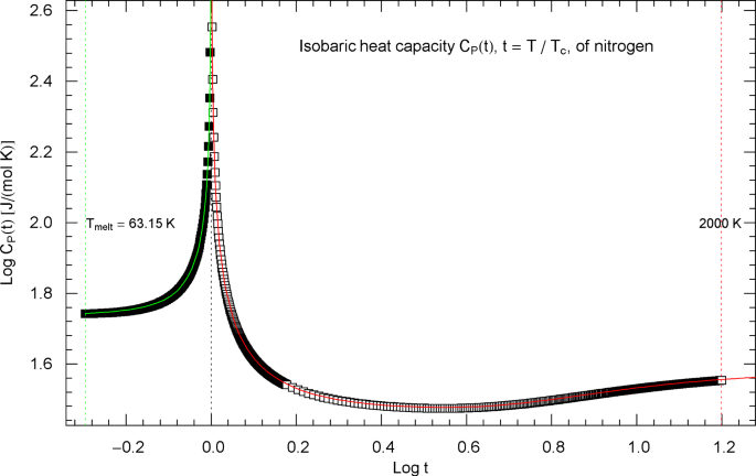
As a first orientation, synthetic experimental data for the isobaric heat capacity $C_{{\text{P}}}$ of nitrogen, cf. Refs. [2, 3], are plotted in Fig. 1, at critical pressure $P_{{\text{c}}} = {3}{\text{.3958 MPa}}$. Figure 1 shows a Log–Log plot of $C_{{\text{P}}}$ data against reduced temperature $t = T/T_{{\text{c}}}$, from the melting point at $T_{{{\text{melt}}}} = {63}{\text{.15 K}}$ up to 125.6 K and from 126.8 K up to 2000 K. (Log denotes the decadic logarithm.) The critical temperature of nitrogen is $T_{{\text{c}}} = {126}{\text{.19 K}}$. Critical point parameters are denoted by $(T_{{\text{c}}} ,P_{{\text{c}}} ,\rho_{{\text{c}}} ,V_{{\text{c}}} )$, where $\rho$ is the molar density and $V = 1/\rho$ the molar volume, cf. Table 1. Despite the pronounced singularity in Fig. 1, the indicated temperature ranges are still by about two orders separated from the scaling regime, where $C_{{\text{P}}} \sim A_{ \pm } \left| {1 - T/T_{{\text{c}}} } \right|^{1/\delta - 1}$ with critical exponent $\delta = 4.7898$, cf. Ref. [27]. The $\pm$ subscripts refer to temperatures above and below $T_{{\text{c}}}$. That is, $C_{{\text{P}}} \sim A_{ + } (t - 1)^{1/\delta - 1}$ for $t > 1$ and $C_{{\text{P}}} \sim A_{ - } (1 - t)^{1/\delta - 1}$ for $t < 1$.

Fig. 1

Isobaric heat capacity of nitrogen at critical pressure. Data points from Refs. [2, 3] (which are synthetic data based on a multiparameter EoS [4]) covering the low-temperature interval from the melting point $T_{{{\text{melt}}}} = {63}{\text{.15 K}}$ to 125.6 K (155 data points, filled squares) and the high-temperature range from 126.8 K up to 2000 K (460 data points, open squares). The critical temperature of nitrogen is $T_{{\text{c}}} = {126}{\text{.19 K}}$. Depicted is a Log–Log (decadic double-logarithmic) plot of the isobaric N₂ heat capacity $C_{{\text{P}}} (t)$ (at the critical pressure of $P_{{\text{c}}} = {3}{\text{.3958 MPa}}$) versus reduced temperature $t = T/T_{{\text{c}}}$. The lower and upper temperature limits are indicated by the vertical green and red dotted lines. The red and green solid curves show least-squares fits to the depicted heat-capacity data. The least-squares regression of the critical heat capacity is performed with the multiply broken power-law densities $C_{{\text{P}}} (\tau )$ in (2.1) (high-temperature branch, $\tau = 1/(t - 1)$, $t > 1$, red solid curve) and (2.5) (low-temperature branch, $\tau = 1/(1 - t)$, $t < 1$, green solid curve) and fitting parameters in Table 2

Table 1 Critical constants (temperature $T_{{\text{c}}}$, molar density $\rho_{{\text{c}}}$, molar volume $V_{{\text{c}}}$, pressure $P_{{\text{c}}}$) and melting point $T_{{{\text{melt}}}}$ of nitrogen, methane, water and hydrogen, cf. Refs. [2, 3]

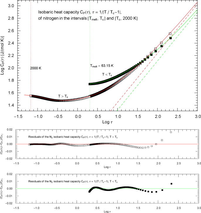
To model the crossover from the empirical data in Fig. 1 to the scaling regime, we parametrize the heat capacity with the scaling variable $\tau = 1/\left| {t - 1} \right|$, $t = T/T_{{\text{c}}}$, writing $C_{{\rm P}} (\tau )$ and splitting the temperature range into a low-temperature interval $[T_{{{\text{melt}}}} ,T_{{\text{c}}} ]$ between melting point and $T_{{\text{c}}}$ and a high-temperature interval above $T_{{\text{c}}}$. Thus, in the low-temperature interval, the scaling variable is $\tau = 1/(1 - t)$, $\tau > 1/(1 - T_{{{\text{melt}}}} /T_{{\text{c}}} )$. In the high-temperature interval, $\tau = 1/(t - 1)$, $\tau > 0$. In either case, the critical temperature $T_{{\text{c}}}$ corresponds to $\tau = \infty$. Figure 2 shows Log–Log plots of the isobaric heat-capacity data (the same as in Fig. 1) as a function of $\tau$ instead of reduced temperature $t = T/T_{{\text{c}}}$. The low-temperature ($T < T_{{\text{c}}}$) data points are depicted as filled squares and the high-temperature ($T > T_{{\text{c}}}$) data as open squares, covering the same temperature range as in Fig. 1.

Fig. 2

Isobaric heat capacity $C_{{\text{P}}} (\tau )$ of nitrogen at critical pressure, parametrized with the scaling variable $\tau = 1/\left| {T/T_{{\text{c}}} - 1} \right|$. The open and filled squares are data points from Refs. [2, 3], the same as depicted in Fig. 1. In the high-temperature regime, $T/T_{{\text{c}}} > 1$, the scaling variable is $\tau = 1/(T/T_{{\text{c}}} - 1)$, and the data points are depicted as open squares. In the low-temperature regime, $T/T_{{\text{c}}} < 1$, the scaling variable is $\tau = 1/(1 - T/T_{{\text{c}}} )$, and the data points are plotted as filled squares. In this $\tau$ parametrization, the critical temperature is mapped to infinity, $\tau (T_{{\text{c}}} ) = \infty$. The red and green solid curves are the high- and low-temperature heat capacities $C_{{\text{P}}} (\tau )$ in (2.1) (for $T > T_{{\text{c}}}$) and (2.5) (for $T < T_{{\text{c}}}$) regressed from the depicted data sets, cf. Table 2 and Sect. 2. The $\chi^{2}$ functional used for the regression is stated in Appendix 1; residuals of the least-squares fits of the high- and low-temperature heat-capacity branches are shown in the lower panels. The red and green dashed lines depicting the critical power-law scaling, cf. (2.2) and (2.6), are the asymptotes of the high- and low-temperature heat capacities $C_{{\text{P}}} (\tau )$ in (2.1) and (2.5). These straight lines have a Log–Log slope of $1 - 1/\delta = 0.7912$, which is the critical exponent of the isobaric heat capacity at critical pressure (of a fluid in the 3D Ising universality class)

2.1 High-temperature regime above the critical temperature

The data set $(\tau_{i} ,C_{{{\text{P}},i}} )$, $\tau_{i} = 1/(T_{i} /T_{{\text{c}}} - 1)$, in the high-temperature regime ($T > T_{{\text{c}}}$) comprises 460 data points in the interval between 126.8 K and 2000 K (open squares in Fig. 2, taken from Refs. [2, 3]).

The least-squares fit above $T_{{\text{c}}}$ is performed with the multiply broken power law, cf. Refs. [28, 29, 37],

$$C_{{\text{P}}} (\tau ) = a_{0} \tau^{{\alpha_{0} }} \frac{1}{{(1 + (\tau /b_{1} )^{{\beta_{1} /\eta_{1} }} )^{{\eta_{1} }} }}(1 + (\tau /b_{2} )^{{\beta_{2} /\eta_{2} }} )^{{\eta_{2} }} (1 + (\tau /b_{3} )^{{\beta_{3} /\eta_{3} }} )^{{\eta_{3} }} ,$$

(2.1)

with positive amplitudes $a_{0}$, $b_{k}$, positive exponents $\beta_{k}$, $\eta_{k}$, and real exponent $\alpha_{0}$ as parameters.

The asymptotic limit of (2.1) is $C_{{\text{P}}} (\tau \to \infty )\sim A_{ + } \tau^{1 - 1/\delta }$, with exponent and amplitude

$$1 - 1/\delta = \alpha_{0} - \beta_{1} + \beta_{2} + \beta_{3} ,\;A_{ + } = a_{0} b_{1}^{{\beta_{1} }} /(b_{2}^{{\beta_{2} }} b_{3}^{{\beta_{3} }} ).$$

(2.2)

We can use the scaling exponent $1 - 1/\delta = 0.7912$ and the first equation in (2.2) to eliminate the parameter $\beta_{3}$ in $C_{{\text{P}}} (\tau )$.

The least-squares regression of $C_{{\text{P}}} (\tau )$ is explained in Appendix 1 and is based on supercritical data points $(\tau_{i} ,C_{{{\text{P}},i}} )_{i = 1,...,N}$, $N = 460$, referenced above. The fitting parameters $a_{0} \,$,$\alpha_{0}$ and $(b_{k} ,\beta_{k} ,\eta_{k} )_{k = 1,2,3}$ are recorded in Table 2, including the amplitude $A_{ + }$ in (2.2). (The decadic logarithm ${\text{Log }}b_{k}$ rather than the amplitude $b_{k}$ is listed in this table.) The regressed high-temperature component (2.1) of the isobaric heat capacity $C_{{\text{P}}} (\tau )$ is depicted in Fig. 2 as red solid curve.

Table 2 Fitting parameters of the high-temperature ($T > T_{{\text{c}}}$) and low-temperature ($T_{{{\text{melt}}}} \le T \le T_{{\text{c}}}$) branches of the isobaric heat capacity at critical pressure $P_{{\text{c}}}$ (cf. Table 1) of nitrogen, methane, water and hydrogen. The nonlinear least-squares regression is explained in Appendix 1. The multiply broken power-law density $C_{{\text{P}}} (\tau )$ for the high-temperature heat-capacity branch of nitrogen (column labeled (${\text{N}}_{2}$, $T > T_{{\text{c}}}$)) reads, cf. (2.1), $C_{{\text{P}}} (\tau ) = a_{0} \tau^{{\alpha_{0} }} (1 + (\tau /b_{1} )^{{\beta_{1} /\eta_{1} }} )^{{ - \eta_{1} }} (1 + (\tau /b_{2} )^{{\beta_{2} /\eta_{2} }} )^{{\eta_{2} }} (1 + (\tau /b_{3} )^{{\beta_{3} /\eta_{3} }} )^{{\eta_{3} }}$. The nitrogen heat capacity at low temperature (column labeled (${\text{N}}_{2}$, $T < T_{{\text{c}}}$)) as well as the methane and water heat-capacity branches at high and low temperature (columns labeled (${\text{CH}}_{4}$,$T > T_{{\text{c}}}$), (${\text{CH}}_{4}$,$T < T_{{\text{c}}}$), (${\text{H}}_{2} {\text{O}}$,$T > T_{{\text{c}}}$) and (${\text{H}}_{2} {\text{O}}$,$T < T_{{\text{c}}}$)) are modeled with the broken power law (2.5), $C_{{\text{P}}} (\tau ) = a_{0} \tau^{{\alpha_{0} }} (1 + (\tau /b_{1} )^{{\beta_{1} /\eta_{1} }} )^{{\eta_{1} }} (1 + (\tau /b_{2} )^{{\beta_{2} /\eta_{2} }} )^{{\eta_{2} }}$. The broken power-law density (5.1) is used for the high-temperature heat-capacity branch of hydrogen (column labeled (${\text{H}}_{2}$,$T > T_{{\text{c}}}$)), $C_{{\text{P}}} (\tau ) = a_{0} \tau^{{\alpha_{0} }} (1 + (\tau /b_{1} )^{{\beta_{1} /\eta_{1} }} )^{{\eta_{1} }} (1 + (\tau /b_{2} )^{{\beta_{2} /\eta_{2} }} )^{{ - \eta_{2} }} (1 + (\tau /b_{3} )^{{\beta_{3} /\eta_{3} }} )^{{\eta_{3} }}$. The regression of the low-temperature heat capacity of hydrogen at critical pressure (column labeled (${\text{H}}_{2}$,$T < T_{{\text{c}}}$)) is based on the broken power law (5.4), $C_{{\text{P}}} (\tau ) = a_{0} \tau^{{\alpha_{0} }} (1 + (\tau /b_{1} )^{{\beta_{1} /\eta_{1} }} )^{{ - \eta_{1} }} (1 + (\tau /b_{2} )^{{\beta_{2} /\eta_{2} }} )^{{\eta_{2} }}$. The broken power laws representing the heat-capacity branches are parametrized with the reciprocal reduced temperature $\tau = 1/\left| {T/T_{{\text{c}}} - 1} \right|$. The least-squares functional used for the regression is stated in (7.6). The data points and the regressed high- and low-temperature heat-capacity branches of nitrogen, methane, water and hydrogen are depicted in Figs. 2, 7, 12 and 17. The fitting parameters $a_{0} [{\text{J}}/({\text{mol K}})], \, \alpha_{0} , \, (b_{k}^{{}} ,\beta_{k}^{{}} ,\eta_{k}^{{}} )$ of the enumerated broken power laws for the respective branches are listed in this table. ${\text{Log }}b_{k}$ denotes the decadic logarithm of the amplitude $b_{k}$, and the amplitude $a_{0}$ is in units of ${\text{J}}/({\text{mol K)}}$; all other parameters are dimensionless. Also recorded are the minimum of the least-squares functional $\chi^{2}$, cf. (7.6), and the degrees of freedom of the fit (dof: number $N$ of data points minus number of fitting parameters). The scaling amplitudes $A_{ \pm }^{{}} [{\text{J}}/({\text{mol K)}}]$ of the critical power laws $C_{{\text{P}}} \sim A_{ + } \tau^{1 - 1/\delta }$ (for the $T > T_{{\text{c}}}$ branch) and $C_{{\text{P}}} \sim A_{ - } \tau^{1 - 1/\delta }$ (for the $T < T_{{\text{c}}}$ branch) are recorded as well. The high- and low-temperature Index curves depicting the Log–Log slope of the critical isobaric heat capacities of nitrogen, methane, water and hydrogen in Figs. 3, 8, 13 and 18, respectively, are also defined by the listed parameters $\alpha_{0} , \, (b_{k}^{{}} ,\beta_{k}^{{}} ,\eta_{k}^{{}} )$

In Fig. 1, the isobaric heat capacity is parametrized with reduced temperature $t = T/T_{{\text{c}}}$. The red solid curve in this figure is the high-temperature $C_{{\text{P}}} (\tau )$ in (2.1) with $\tau = 1/(t - 1)$ substituted (shortcut $C_{{\text{P}}} (t)$).

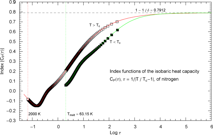
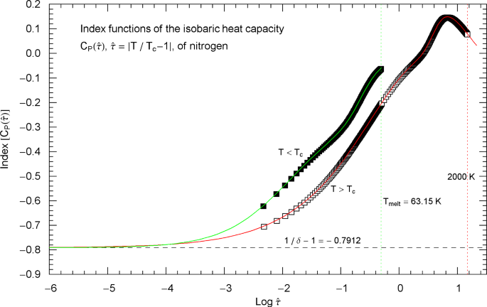
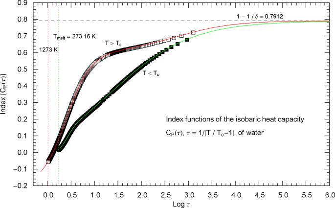
Figure 3 depicts the Index function, cf., e.g., Refs. [30, 35, 38,39,40,41],

$${\text{Index[}}C_{{\text{P}}} (\tau )]: = \frac{{C^{\prime}_{{\text{P}}} (\tau )}}{{C_{{\text{P}}} (\tau )}}\tau = \frac{{{\text{d}}\log C_{{\text{P}}} (\tau )}}{{{\text{d}}\log \tau }},$$

(2.3)

i.e., the Log–Log slope (red solid curve) of the regressed high-temperature heat capacity $C_{{\text{P}}} (\tau )$ in (2.1),

$${\text{Index[}}C_{{\text{P}}} (\tau )] = \alpha_{0} - \beta_{1} \frac{{(\tau /b_{1} )^{{\beta_{1} /\eta_{1} }} }}{{1 + (\tau /b_{1} )^{{\beta_{1} /\eta_{1} }} }} + \beta_{2} \frac{{(\tau /b_{2} )^{{\beta_{2} /\eta_{2} }} }}{{1 + (\tau /b_{2} )^{{\beta_{2} /\eta_{2} }} }} + \beta_{3} \frac{{(\tau /b_{3} )^{{\beta_{3} /\eta_{3} }} }}{{1 + (\tau /b_{3} )^{{\beta_{3} /\eta_{3} }} }}.$$

(2.4)

Fig. 3

Index functions of the critical isobaric heat capacity of nitrogen, parametrized with scaling variable $\tau = 1/\left| {T/T_{{\text{c}}} - 1} \right|$. The red and green solid curves show the Log–Log slope ${\text{Index[}}C_{{\text{P}}} (\tau )]: = {\text{d}}\log C_{{\text{P}}} (\tau )/{\text{d}}\log \tau$ of the high- and low-temperature heat-capacity branches $C_{{\text{P}}} (\tau )$ of nitrogen, cf. Section 2. Log–Log plots of $C_{{\text{P}}} (\tau )$, cf. (2.1) (for $T > T_{{\text{c}}}$) and (2.5) (for $T < T_{{\text{c}}}$), are depicted in Fig. 2 as red and green solid curves. The plotted Index functions ${\text{Index[}}C_{{\text{P}}} (\tau )]$ are stated in (2.4) (red solid curve, $\tau = 1/(T/T_{{\text{c}}} - 1)$, $T > T_{{\text{c}}}$) and (2.7) (green solid curve, $\tau = 1/(1 - T/T_{{\text{c}}} )$, $T < T_{{\text{c}}}$) with parameters in Table 2. The open squares on the (red solid) high-temperature ($T > T_{{\text{c}}}$) Index curve and the filled squares on the (green solid) low-temperature ($T < T_{{\text{c}}}$) Index curve correspond to the heat-capacity data points depicted in Fig. 2. The vertical red and green dotted lines indicate the same temperature intervals as in Fig. 2. The scaling exponent $1 - 1/\delta = 0.7912$ of the heat capacity is indicated by the black dashed horizontal line, which is the asymptote of the depicted Index curves (i.e., the constant $\tau \to \infty$ limit of ${\text{Index[}}C_{{\text{P}}} (\tau )]$ in (2.4) and (2.7)). This horizontal line is also a plot of the constant Index function (Log–Log slope) of the asymptotes of the heat-capacity branches $C_{{\text{P}}} (\tau )$ in Fig. 2 (red and green dashed straight lines in Fig. 2, depicting the asymptotic power laws (2.2) and (2.6) of the isobaric heat capacity at critical pressure)

To better relate Figs. 2 and 3, we have plotted data points $(\tau_{i} ,{\text{Index[}}C_{{\text{P}}} (\tau_{i} )])_{i = 1,...,N}$ (open squares) on the Index curve, using the abscissas $\tau_{i}$ of the data points $(\tau_{i} ,C_{{{\text{P}},i}} )_{i = 1,...,N}$ in Fig. 2 (also indicated by open squares).

2.2 Low-temperature interval between melting point and critical temperature

The data set $(\tau_{i} ,C_{{{\text{P}},i}} )$ used for the regression of the isobaric heat capacity $C_{{\text{P}}} (\tau )$ at critical pressure in the subcritical interval $[T_{{{\text{melt}}}} ,T_{{\text{c}}} ]$ comprises 155 data points between $T_{{{\text{melt}}}} = 63.15{\text{ K}}$ and 125.6 K (filled squares in Fig. 2, taken from Refs. [2, 3]).

The least-squares fit of the low-temperature branch of $C_{{\text{P}}} (\tau )$ is performed with the broken power law

$$C_{{\text{P}}} (\tau ) = a_{0} \tau^{{\alpha_{0} }} (1 + (\tau /b_{1} )^{{\beta_{1} /\eta_{1} }} )^{{\eta_{1} }} (1 + (\tau /b_{2} )^{{\beta_{2} /\eta_{2} }} )^{{\eta_{2} }} .$$

(2.5)

The amplitudes $a_{0}$, $b_{k}$ and exponents $\beta_{k}$, $\eta_{k}$ are positive, and the exponent $\alpha_{0}$ is real. The asymptotic power-law scaling of $C_{{\text{P}}} (\tau )$ in (2.5) reads $C_{{\text{P}}} (\tau \to \infty )\sim A_{ - } \tau^{1 - 1/\delta }$, with

$$1 - 1/\delta = \alpha_{0} + \beta_{1} + \beta_{2} ,\;A_{ - } = a_{0} /(b_{1}^{{\beta_{1} }} b_{2}^{{\beta_{2} }} ).$$

(2.6)

The exponent $\beta_{2}$ in (2.5) can be eliminated via the first identity in (2.6), using the calculated scaling exponent $1 - 1/\delta = 0.7912$.

The least-squares regression of $C_{{\text{P}}} (\tau )$ in (2.5) is analogous to the regression of the high-temperature component of the heat capacity in Sect. 2.1, based on the subcritical data set $(\tau_{i} ,C_{{{\text{P}},i}} )_{i = 1,...,N}$, $\tau_{i} = 1/(1 - t_{i} )$, $N = 155$, referenced above. The fitting parameters $a_{0} , \, \alpha_{0}$, $(b_{k}^{{}} ,\beta_{k}^{{}} ,\eta_{k}^{{}} )_{k = 1,2}$ are listed in Table 2, as well as the amplitude $A_{ - }$ in (2.6). The regressed $C_{{\text{P}}} (\tau )$ is shown in Fig. 2 as green solid curve. The red and green straight lines in Fig. 2 depict the asymptotic power-law scaling $C_{{\text{P}}} \sim A_{ \pm } \tau^{1 - 1/\delta }$. In Fig. 1, $C_{{\text{P}}} (\tau = 1/(1 - t))$ is plotted as a function of reduced temperature $t = T/T_{{\text{c}}} < 1$ (green solid curve in Fig. 1).

The Index function of the low-temperature heat capacity $C_{{\text{P}}} (\tau )$ in (2.5) is depicted in Fig. 3 as green solid curve,

$${\text{Index[}}C_{{\rm P}} (\tau )] = \alpha_{0} + \beta_{1} \frac{{(\tau /b_{1} )^{{\beta_{1} /\eta_{1} }} }}{{1 + (\tau /b_{1} )^{{\beta_{1} /\eta_{1} }} }} + \beta_{2} \frac{{(\tau /b_{2} )^{{\beta_{2} /\eta_{2} }} }}{{1 + (\tau /b_{2} )^{{\beta_{2} /\eta_{2} }} }},$$

(2.7)

which is the Log–Log slope of the low-temperature branch of the heat capacity $C_{{\text{P}}} (\tau )$ in Fig. 2. Along the Index curve in Fig. 3, we have indicated data points $(\tau_{i} ,{\text{Index[}}C_{{\rm P}} (\tau_{i} )])_{i = 1,...,N}$ (filled squares) with the same abscissas as the low-temperature points $(\tau_{i} ,C_{{{\text{P}},i}} )_{i = 1,...,N}$ in Fig. 2.

Outside the interval $[125.6{\text{ K}}, \, 1{26}{\text{.8 K}}]$, the Index functions in Fig. 3 do not exceed 0.7. The complement of this interval is covered by the open and filled squares in Figs. 2 and 3, representing synthetic data sets of the critical isobaric N₂ heat capacity from Refs. [2, 3]. The slope of $1 - 1/\delta = 0.7912$ exhibiting the critical power-law scaling of the isobaric heat capacity is only reached for temperatures extremely close to $T_{{\text{c}}} = 126.19{\text{ K}}$, $\left| {T/T_{{\text{c}}} - 1} \right| < 10^{ - 5}$, see Fig. 3 (where $T_{{\text{c}}}$ corresponds to $\tau = \infty$), far outside the temperature range of the empirical data.

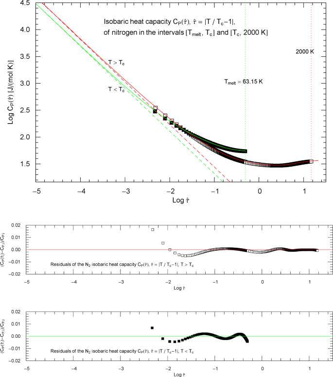
Figure 4 shows the heat-capacity branches $C_{{\rm P}} (\hat{\tau })$ in reduced-temperature parametrization, $\hat{\tau } = \left| {t - 1} \right|$, $t = T/T_{{\text{c}}}$, and is otherwise analogous to Fig. 2. The red and green straight lines in Fig. 4 depict the asymptotic power-law scaling $C_{{\text{P}}} \sim A_{ \pm } \hat{\tau }^{1/\delta - 1}$. The Index curves ${\text{Index[}}C_{{\text{P}}} (\hat{\tau })]$ of the high- and low-temperature heat-capacity branches in reduced-temperature parametrization are plotted in Fig. 5.

Fig. 4

Isobaric heat capacity $C_{{\text{P}}} (\hat{\tau })$ of nitrogen at critical pressure, parametrized with reduced temperature $\hat{\tau } = \left| {T/T_{{\text{c}}} - 1} \right|$. Apart from this reparametrization, the caption of Fig. 2 is applicable. In this $\hat{\tau }$ parametrization, the critical temperature is mapped to zero. The red and green solid curves show the high- and low-temperature heat-capacity branches $C_{{\text{P}}} (\tau = 1/\hat{\tau })$ in (2.1) (for $T > T_{{\text{c}}}$) and (2.5) (for $T < T_{{\text{c}}}$) regressed from the depicted data sets, cf. Section 2 and Table 2. The residuals of the least-squares fits of the high- and low-temperature branches are shown in the lower panels, indicating deviations of less than one percent throughout the data range. The red and green dashed lines depicting the critical power laws $C_{{\text{P}}} (\hat{\tau } \to 0)\sim A_{ \pm } \hat{\tau }^{1/\delta - 1}$, cf. (2.2) and (2.6), are the asymptotes of the high- and low-temperature branches of $C_{{\text{P}}} (\hat{\tau })$

Fig. 5

Index functions of the isobaric heat capacity of nitrogen at critical pressure, parametrized with reduced temperature $\hat{\tau } = \left| {T/T_{{\text{c}}} - 1} \right|$. The red and green solid curves depict the Log–Log slope ${\text{Index[}}C_{{\rm P}} (\tau = 1/\hat{\tau })] = - {\text{Index[}}C_{{\rm P}} (\tau )]|_{{\tau = 1/\hat{\tau }}}$ of the high- and low-temperature branches of the nitrogen heat capacity $C_{{\rm P}} (\hat{\tau })$ in Fig. 4, cf. (2.1), (2.5). The Index functions are stated in (2.4) and (2.7), subject to the substitution $\tau = 1/\hat{\tau }$ and an overall sign change as indicated. The open squares on the (red solid) high-temperature ($T > T_{{\text{c}}}$) Index curve and the filled squares on the (green solid) low-temperature ($T < T_{{\text{c}}}$) Index curve correspond to the heat-capacity data points in Fig. 4. The scaling exponent $1 - 1/\delta = 0.7912$ of the isobaric heat capacity at critical pressure is indicated by the black dashed horizontal line, which is the asymptote of the depicted Index curves. This horizontal line is also a plot of the constant Index function (Log–Log slope) of the critical power laws $A_{ \pm } \hat{\tau }^{1/\delta - 1}$ asymptotic to the high- and low-temperature branches of $C_{{\text{P}}} (\hat{\tau })$ in Fig. 4. (These asymptotes are depicted as red and green dashed straight lines in Fig. 4)

3 Critical isobaric heat capacity of methane

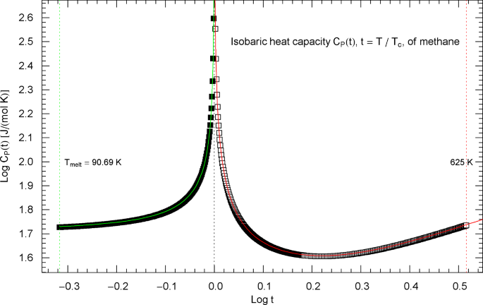
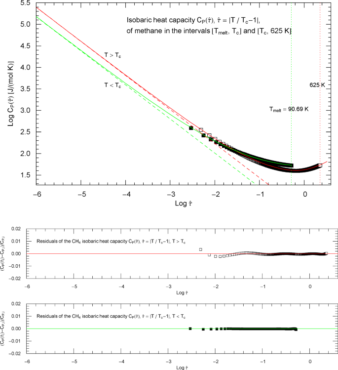
The reasoning in this section and Sect. 4 (heat capacity of water) is quite analogous to the discussion of the nitrogen heat capacity in Sect. 2. Experimental data for the isobaric heat capacity of methane, cf. Refs. [2, 3], are plotted in Fig. 6, at critical pressure $P_{{\text{c}}} = {4}{\text{.5992 MPa}}$. Figure 6 shows a Log–Log plot of $C_{{\rm P}}$ data against reduced temperature $t = T/T_{{\text{c}}}$, from the melting point at $T_{{{\text{melt}}}} = {90}{\text{.694 K}}$ up to 190 K and from 191.5 K up to 625 K. The critical temperature of methane is $T_{{\text{c}}} = {190}{\text{.56 K}}$, cf. Table 1.

Fig. 6

Isobaric heat capacity of methane at critical pressure. Data points from Refs. [2, 3] (which are synthetic data based on a multiparameter EoS [5]), covering the low-temperature interval from the melting point $T_{{{\text{melt}}}} = {90}{\text{.694 K}}$ up to 190 K (197 data points, filled squares) and the high-temperature range from 191.5 K to 625 K (366 data points, open squares). The critical temperature of methane is $T_{{\text{c}}} = {190}{\text{.56 K}}$. Depicted is a Log–Log (decadic double-logarithmic) plot of the isobaric CH₄ heat capacity $C_{{\text{P}}} (t)$ (at the critical pressure of $P_{{\text{c}}} = {4}{\text{.5992 MPa}}$) in reduced temperature $t = T/T_{{\text{c}}}$. The lower and upper temperature limits are indicated by the vertical green and red dotted lines. The red and green solid curves show least-squares fits to the depicted heat-capacity data. Both the high-temperature branch ($t > 1$, red solid curve) and low-temperature branch ($T_{{{\text{melt}}}} /T_{{\text{c}}} < t < 1$, green solid curve) of the heat capacity are modeled with the broken power-law density $C_{{\text{P}}} (\tau )$ in (2.5), with $\tau = 1/\left| {t - 1} \right|$ substituted, cf. Section 3. The fitting parameters of the high- and low-temperature branches of the critical isobaric CH₄ heat capacity are recorded in Table 2

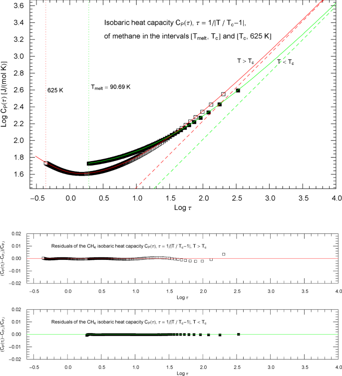
To model the crossover from the empirical data in Fig. 6 to the scaling regime (where $C_{{\text{P}}} \sim A_{ \pm } \left| {1 - T/T_{{\text{c}}} } \right|^{ 1/\delta - 1 }$ and $1 - 1/\delta = 0.7912$), we parametrize the heat capacity with the scaling variable $\tau = 1/\left| {t - 1} \right|$, $t = T/T_{{\text{c}}}$. Figure 7 shows Log–Log plots of the isobaric heat-capacity data as a function of $\tau$. The low-temperature ($T < T_{{\text{c}}}$) data points are depicted as filled squares and the high-temperature ($T > T_{{\text{c}}}$) data as open squares, covering the same temperature range as in Fig. 6.

Fig. 7

Isobaric heat capacity $C_{{\text{P}}} (\tau )$ of methane at critical pressure, parametrized with the scaling variable $\tau = 1/\left| {T/T_{{\text{c}}} - 1} \right|$. The open and filled squares are data points from Refs. [2, 3], the same as depicted in Fig. 6. In the high-temperature regime, $T/T_{{\text{c}}} > 1$, the scaling variable is $\tau = 1/(T/T_{{\text{c}}} - 1)$, and the data points are depicted as open squares. In the low-temperature regime, $T/T_{{\text{c}}} < 1$, the scaling variable is $\tau = 1/(1 - T/T_{{\text{c}}} )$, and the data points are shown as filled squares. The red and green solid curves are the high- and low-temperature heat capacities $C_{{\text{P}}} (\tau )$ in (2.5) (for $T > T_{{\text{c}}}$ and $T_{{{\text{melt}}}} < T < T_{{\text{c}}}$, respectively) regressed from the depicted data sets, cf. Table 2. The $\chi^{2}$ functional used for the regression is stated in (7.6), and the residuals of the least-squares fits of the high- and low-temperature branches of the CH₄ heat capacity are shown in the lower panels. The red and green dashed lines are the asymptotes of the high- and low-temperature branches (red and green solid curves), cf. Section 3. These straight lines depict simple power laws and have a Log–Log slope of $1 - 1/\delta = 0.7912$ coinciding with the scaling exponent of the critical isobaric heat capacity

3.1 Heat capacity as broken power law: high-temperature interval from $T_{{\text{c}}}$ up to 625 K

The data set $(\tau_{i} ,C_{{{\text{P}},i}} )$, $\tau_{i} = 1/(T_{i} /T_{{\text{c}}} - 1)$, used for regression in the high-temperature regime ($T > T_{{\text{c}}}$) comprises 366 data points in the interval between 191.5 K and 625 K (open squares in Fig. 7, cf. Refs. [2, 3]).

The least-squares fit above $T_{{\text{c}}}$ is performed with the broken power law $C_{{\text{P}}} (\tau )$ already stated in (2.5), with positive amplitudes $a_{0}$, $b_{k}$, positive exponents $\beta_{k}$, $\eta_{k}$, and real exponent $\alpha_{0}$ as parameters. The asymptotic limit of the broken power law (2.5) is $C_{{\text{P}}} (\tau \to \infty )\sim A_{ + } \tau^{1 - 1/\delta }$, with exponent $1 - 1/\delta = \alpha_{0} + \beta_{1} + \beta_{2}$ and amplitude $A_{ + } = a_{0} /(b_{1}^{{\beta_{1} }} b_{2}^{{\beta_{2} }} )$, cf. (2.6). We use the scaling exponent $1 - 1/\delta = 0.7912$ and eliminate the exponent $\beta_{2}$ of $C_{{\text{P}}} (\tau )$ in (2.5) by substituting $\beta_{2} = 0.7912 - \alpha_{0} - \beta_{1}$.

The least-squares regression of $C_{{\text{P}}} (\tau )$ in (2.5) (with the indicated constraints) is based on supercritical data points $(\tau_{i} ,C_{{{\text{P}},i}} )_{i = 1,...,N}$, $N = 366$, referenced above. The fitting parameters $a_{0} \,$,$\alpha_{0}$, $(b_{k}^{{}} ,\beta_{k}^{{}} ,\eta_{k}^{{}} )_{k = 1,2}$ are recorded in Table 2. The regressed high-temperature branch (2.5) of the isobaric heat capacity $C_{{\text{P}}} (\tau )$ of methane is depicted in Fig. 7 as red solid curve.

In Fig. 6, the isobaric heat capacity is parametrized with reduced temperature $t = T/T_{{\text{c}}}$. The red solid curve in this figure is the regressed high-temperature $C_{{\text{P}}} (\tau )$ in (2.5) and Table 2 with $\tau = 1/(t - 1)$ substituted (shortcut $C_{{\text{P}}} (t)$). The data points in Figs. 6 and 7 are identical.

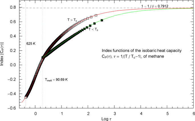
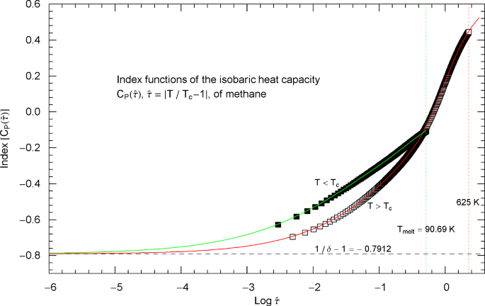
Figure 8 shows the Index function (2.7), i.e., the Log–Log slope (red solid curve) of the regressed high-temperature heat capacity $C_{{\text{P}}} (\tau )$ of methane. To relate Figs. 7 and 8, we have plotted data points $(\tau_{i} ,{\text{Index[}}C_{{\text{P}}} (\tau_{i} )])_{i = 1,...,N}$ (open squares) on the Index curve, using the abscissas $\tau_{i}$ of the data points $(\tau_{i} ,C_{{{\text{P}},i}} )_{i = 1,...,N}$ in Fig. 7.

Fig. 8

Index functions of the critical isobaric heat capacity of methane, parametrized with scaling variable $\tau = 1/\left| {T/T_{{\text{c}}} - 1} \right|$. The red and green solid curves show the Log–Log slope ${\text{Index[}}C_{{\text{P}}} (\tau )] = {\text{d}}\log C_{{\text{P}}} (\tau )/{\text{d}}\log \tau$ of the high- and low-temperature heat-capacity branches $C_{{\text{P}}} (\tau )$ of methane at critical pressure, cf. Section 3. Log–Log plots of the high- and low-temperature branches, cf. (2.5), are depicted in Fig. 7 as red and green solid curves (for $T > T_{{\text{c}}}$ and $T < T_{{\text{c}}}$), respectively. The Index functions ${\text{Index[}}C_{{\text{P}}} (\tau )]$ are stated in (2.7) and plotted here as red solid curve (with $\tau = 1/(T/T_{{\text{c}}} - 1)$, $T > T_{{\text{c}}}$) and green solid curve (with $\tau = 1/(1 - T/T_{{\text{c}}} )$, $T < T_{{\text{c}}}$). The parameters of the high- and low-temperature CH₄ Index functions (2.7) are recorded in Table 2. The open squares along the (red solid) high-temperature Index curve and the filled squares along the (green solid) low-temperature Index curve correspond to the heat-capacity data points in Fig. 7. The vertical red and green dotted lines indicate the same temperature intervals as in Fig. 7. The scaling exponent $1 - 1/\delta = 0.7912$ of the critical isobaric heat capacity is indicated by the black dashed horizontal line, which is the asymptote of the depicted Index curves (i.e., the constant $\tau \to \infty$ limit of ${\text{Index[}}C_{{\text{P}}} (\tau )]$ in (2.7)). This horizontal line is also a plot of the constant Index function (Log–Log slope) of the asymptotes of the high- and low-temperature branches of $C_{{\text{P}}} (\tau )$, depicted as red and green dashed straight lines in Fig. 7

3.2 Regression of the heat capacity in the interval $[T_{{{\text{melt}}}} ,T_{{\text{c}}} ]$

The data set $(\tau_{i} ,C_{{{\text{P}},i}} )$ used for the regression of the isobaric heat capacity $C_{{\text{P}}} (\tau )$ at critical pressure in the subcritical interval $[T_{{{\text{melt}}}} ,T_{{\text{c}}} ]$ comprises 197 data points between $T_{{{\text{melt}}}} = {90}{\text{.694 K}}$ and 190 K (filled squares in Fig. 7, from Refs. [2, 3]).

The least-squares fit of the low-temperature branch of $C_{{\text{P}}} (\tau )$ is also performed with the broken power law $C_{{\text{P}}} (\tau )$ (2.5), subject to the constraints (2.6). The exponent $\beta_{2}$ of $C_{{\text{P}}} (\tau )$ is eliminated by way of the first identity in (2.6). The least-squares regression of $C_{{\text{P}}} (\tau )$ in (2.5) is based on subcritical data points $(\tau_{i} ,C_{{{\text{P}},i}} )_{i = 1,...,N}$, $N = 197$, referenced above. The fitting parameters $a_{0}$,$\alpha_{0}$, $(b_{k}^{{}} ,\beta_{k}^{{}} ,\eta_{k}^{{}} )_{k = 1,2}$ and the amplitude $A_{ - }$ in (2.6) are recorded in Table 2. The regressed low-temperature ($T < T_{{\text{c}}}$) heat capacity $C_{{\text{P}}} (\tau )$ of methane is shown in Fig. 7 as green solid curve. The red and green straight lines in Fig. 7 depict the asymptotic power-law scaling $C_{{\text{P}}} \sim A_{ \pm } \tau^{1 - 1/\delta }$ of the high- and low-temperature branches of the isobaric heat capacity. In Fig. 6, $C_{{\text{P}}} (\tau = 1/(1 - t))$ is plotted as a function of reduced temperature $t = T/T_{{\text{c}}} < 1$ (shortcut $C_{{\text{P}}} (t)$, green solid curve in Fig. 6).

The Index function (2.7) (i.e., Log–Log slope) of the low-temperature heat capacity $C_{{\text{P}}} (\tau )$ in (2.5) and Fig. 7 is depicted in Fig. 8 as green solid curve. On this Index curve in Fig. 8, we have indicated data points $(\tau_{i} ,{\text{Index[}}C_{{\text{P}}} (\tau_{i} )])_{i = 1,...,N}$ (filled squares) with the same abscissas as the subcritical data points $(\tau_{i} ,C_{{{\text{P}},i}} )_{i = 1,...,N}$ in Fig. 7 (also depicted by filled squares).

Outside the interval $[190{\text{ K}}, \, 1{91}{\text{.5 K}}]$, the Index functions in Fig. 8 do not exceed 0.7. The complement of this interval is covered by the open and filled squares in Figs. 7 and 8, representing empirical data sets of the critical isobaric CH₄ heat capacity from Refs. [2, 3]. The Log–Log slope of $1 - 1/\delta = 0.7912$ defining the critical power-law scaling of the isobaric heat capacity at critical pressure is only reached for temperatures extremely close to $T_{{\text{c}}} = {190}{\text{.56 K}}$, in the interval $\left| {T/T_{{\text{c}}} - 1} \right| < 10^{ - 5}$, cf. Fig. 8, far outside the temperature range of the empirical data of Refs. [2, 3]. Figures 9 and 10 show the high- and low-temperature heat capacities and their Index functions in reduced-temperature parametrization, $\hat{\tau } = \left| {t - 1} \right|$, $t = T/T_{{\text{c}}}$, and are otherwise analogous to Figs. 7 and 8. The red and green straight lines in Fig. 9 depict the asymptotic power-law scaling $C_{{\text{P}}} \sim A_{ \pm } \hat{\tau }^{1/\delta - 1}$.

Fig. 9

Isobaric heat capacity $C_{{\text{P}}} (\hat{\tau })$ of methane at critical pressure, parametrized with reduced temperature $\hat{\tau } = \left| {T/T_{{\text{c}}} - 1} \right|$. Apart from this reparametrization, the caption of Fig. 7 applies. The red and green solid curves show the high- and low-temperature heat-capacity branches $C_{{\text{P}}} (\tau = 1/\hat{\tau })$ in (2.5) and Table 2, regressed from the depicted data sets, cf. Section 3. The residuals of the least-squares fits of the high- and low-temperature branches of $C_{{\text{P}}} (\hat{\tau })$ are shown in the lower panels, indicating deviations of less than one percent from the data points. The parallel red and green dashed straight lines depicting the critical power laws $C_{{\text{P}}} (\hat{\tau } \to 0)\sim A_{ \pm } \hat{\tau }^{1/\delta - 1}$ are the asymptotes of the high- and low-temperature branches of $C_{{\text{P}}} (\hat{\tau })$

Fig. 10

Index functions of the isobaric heat capacity of methane at critical pressure, parametrized with reduced temperature $\hat{\tau } = \left| {T/T_{{\text{c}}} - 1} \right|$. The red and green solid curves depict the Log–Log slope ${\text{Index[}}C_{{\text{P}}} (\tau = 1/\hat{\tau })] = - {\text{Index[}}C_{{\text{P}}} (\tau )]|_{{\tau = 1/\hat{\tau }}}$ of the high- and low-temperature branches of the methane heat capacity $C_{{\text{P}}} (\hat{\tau })$ in Fig. 9. The Index functions are defined in (2.7) and Table 2, subject to the substitution $\tau = 1/\hat{\tau }$ and an overall sign change as indicated. The open squares on the high-temperature ($T > T_{{\text{c}}}$) Index curve and the filled squares on the low-temperature ($T < T_{{\text{c}}}$) Index curve correspond to the data points depicted in Fig. 9. The scaling exponent $1 - 1/\delta = 0.7912$ of the isobaric heat capacity at critical pressure is indicated by the black dashed horizontal line, which is the asymptote of the Index curves. This horizontal line is also a plot of the constant Index function (Log–Log slope) of the critical power laws $A_{ \pm } \hat{\tau }^{1/\delta - 1}$ asymptotic to the high- and low-temperature branches of $C_{{\text{P}}} (\hat{\tau })$ in Fig. 9. These power laws are depicted as parallel red and green dashed straight lines in Fig. 9

4 Critical isobaric heat capacity of water

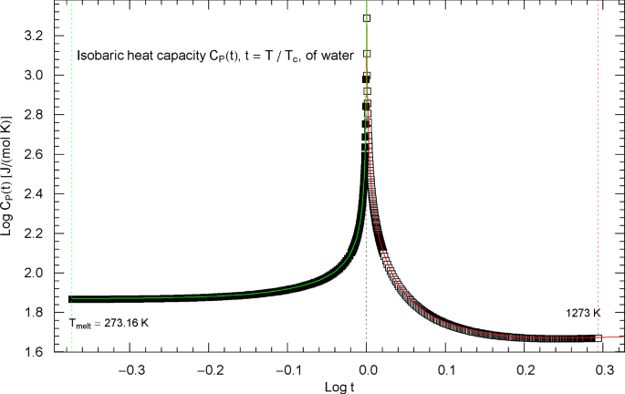
Experimental data for the isobaric heat capacity of water, cf. Refs. [2, 3], are plotted in Fig. 11, at critical pressure of $P_{{\text{c}}} = {22}{\text{.064 MPa}}$. Figure 11 shows a Log–Log plot of the $C_{{\rm P}}$ data sets against reduced temperature $t = T/T_{{\text{c}}}$, from the melting point at $T_{{{\text{melt}}}} = {273}{\text{.16 K}}$ up to 646.4 K and from 647.6 K to 1273 K. The critical temperature of water is $T_{{\text{c}}} = {647}{\text{.10 K}}$, cf. Table 2.

Fig. 11

Isobaric heat capacity of water at critical pressure. Data points from Refs. [2, 3] (synthetic data based on a multiparameter EoS [6]), covering the low-temperature interval from the melting point $T_{{{\text{melt}}}} = {273}{\text{.16 K}}$ to 646.4 K (183 data points, filled squares) and the high-temperature range from 647.6 K to 1273 K (280 data points, open squares). The critical temperature of water is $T_{{\text{c}}} = {647}{\text{.10 K}}$. Depicted is a Log–Log plot of the isobaric heat capacity $C_{{\rm P}} (t)$ (at the critical pressure of $P_{{\text{c}}} = {22}{\text{.064 MPa}}$) versus reduced temperature $t = T/T_{{\text{c}}}$. The lower and upper temperature limits are indicated by the vertical green and red dotted lines. The red and green solid curves show least-squares fits to the depicted heat-capacity data. Both the high-temperature branch ($t > 1$, red solid curve) and low-temperature branch ($T_{{{\text{melt}}}} /T_{{\text{c}}} < t < 1$, green solid curve) of the heat capacity are modeled with the multiply broken power-law density $C_{{\text{P}}} (\tau )$ in (2.5), with $\tau = 1/\left| {t - 1} \right|$ substituted, cf. Section 4. The fitting parameters of the high- and low-temperature branches of the critical isobaric heat capacity of water are recorded in Table 2

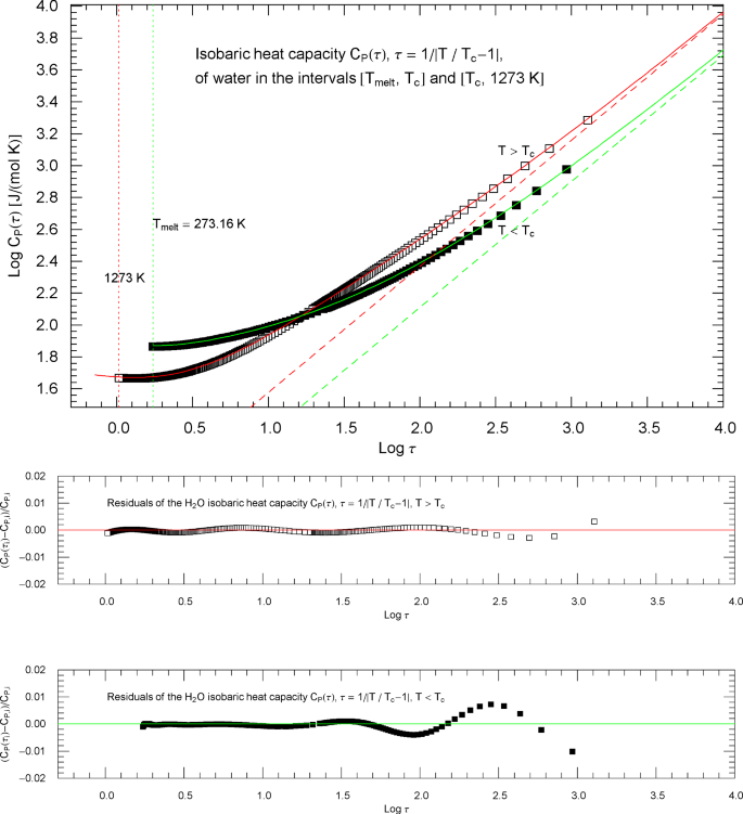
To model the crossover from the empirical data in Fig. 11 to the scaling regime, we parametrize the heat capacity with the scaling variable $\tau = 1/\left| {t - 1} \right|$. Figure 12 shows Log–Log plots of the heat-capacity data as a function of $\tau$. The low-temperature ($T < T_{{\text{c}}}$) data points are depicted as filled squares and the high-temperature ($T > T_{{\text{c}}}$) data as open squares, covering the same temperature range as in Fig. 11. $T_{{\text{c}}}$ in Fig. 11 corresponds to $\tau = \infty$ in Fig. 12.

Fig. 12

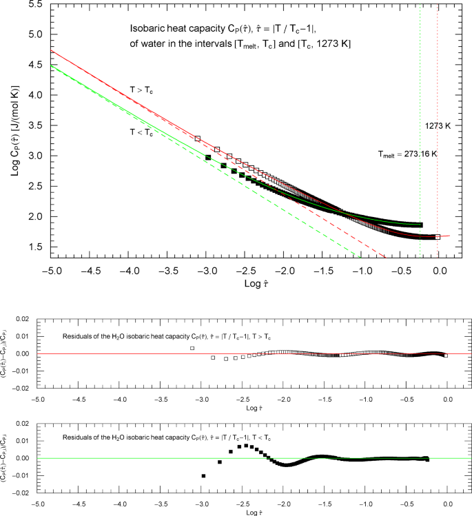
Isobaric heat capacity $C_{{\text{P}}} (\tau )$ of water at critical pressure, parametrized with the scaling variable $\tau = 1/\left| {T/T_{{\text{c}}} - 1} \right|$. The open and filled squares are data points from Refs. [2, 3], the same as depicted in Fig. 11. In the high-temperature regime, $T/T_{{\text{c}}} > 1$, the scaling variable is $\tau = 1/(T/T_{{\text{c}}} - 1)$, and the data points are shown as open squares. In the low-temperature regime, $T/T_{{\text{c}}} < 1$, the scaling variable is $\tau = 1/(1 - T/T_{{\text{c}}} )$, and the data points are plotted as filled squares. In this $\tau$ parametrization, the critical temperature is mapped to infinity. The red and green solid curves are the high- and low-temperature heat capacities $C_{{\rm P}} (\tau )$ in (2.5) (for $T > T_{{\text{c}}}$ and $T_{{{\text{melt}}}} < T < T_{{\text{c}}}$, respectively) regressed from the depicted data sets, cf. Table 2 and Sect. 4. The $\chi^{2}$ functional used for the regression is stated in (7.6); residuals of the least-squares fits of the high- and low-temperature heat-capacity branches are shown in the lower panels. The red and green dashed lines are the asymptotes of the high- and low-temperature branches (red and green solid curves). These straight lines depicting the critical power laws have a Log–Log slope of $1 - 1/\delta = 0.7912$, which is the scaling exponent of the isobaric heat capacity at critical pressure

4.1 Analytic closed-form modeling of the heat capacity at critical pressure: high-temperature regime from $T_{{\text{c}}}$ to 1270 K

The data set $(\tau_{i} ,C_{{{\text{P}},i}} )$, $\tau_{i} = 1/(T_{i} /T_{{\text{c}}} - 1)$, in the high-temperature regime ($T > T_{{\text{c}}}$) comprises 280 data points in the interval between 647.6 K and 1273 K (open squares in Fig. 10, cf. Refs. [2, 3]). The least-squares fit above $T_{{\text{c}}}$ is performed with the broken power law $C_{{\text{P}}} (\tau )$ in (2.5), with positive amplitudes $a_{0}$, $b_{k}$, positive exponents $\beta_{k}$, $\eta_{k}$, and real exponent $\alpha_{0}$ as parameters. The asymptotic limit of the broken power law (2.5) is $C_{{\text{P}}} (\tau \to \infty )\sim A_{ + } \tau^{1 - 1/\delta }$, with exponent $1 - 1/\delta = \alpha_{0} + \beta_{1} + \beta_{2}$ and amplitude $A_{ + } = a_{0} /(b_{1}^{{\beta_{1} }} b_{2}^{{\beta_{2} }} )$. We use the calculated scaling exponent $1 - 1/\delta = 0.7912$ and eliminate the exponent $\beta_{2}$ in $C_{{\text{P}}} (\tau )$ by way of the first identity.

The least-squares regression of $C_{{\text{P}}} (\tau )$ in (2.5) is based on supercritical data points $(\tau_{i} ,C_{{{\text{P}},i}} )_{i = 1,...,N}$, $N = 280$, referenced above. The fitting parameters $a_{0}$,$\alpha_{0}$,$(b_{k}^{{}} ,\beta_{k}^{{}} ,\eta_{k}^{{}} )_{k = 1,2}$ and the derived asymptotic amplitude $A_{ + }$ are recorded in Table 2. The regressed high-temperature branch (2.5) of the isobaric heat capacity $C_{{\text{P}}} (\tau )$ of water is depicted in Fig. 12 as red solid curve.

Figure 11 depicts the critical isobaric heat capacity of water parametrized with reduced temperature $t = T/T_{{\text{c}}}$. The red solid curve in this figure shows $C_{{\text{P}}} (\tau )$ in (2.5) with $\tau = 1/(t - 1)$ substituted (shortcut $C_{{\text{P}}} (t)$).

Figure 13 depicts the Index function (2.7) (red solid curve), i.e., the Log–Log slope of the regressed high-temperature heat capacity $C_{{\text{P}}} (\tau )$ in Fig. 12. To relate Figs. 12 and 13, we have plotted data points $(\tau_{i} ,{\text{Index[}}C_{{\text{P}}} (\tau_{i} )])_{i = 1,...,N}$ (open squares) on the Index curve, using the abscissas $\tau_{i}$ of the supercritical data points $(\tau_{i} ,C_{{{\text{P}},i}} )_{i = 1,...,N}$ in Fig. 12 (also indicated by open squares).

Fig. 13

Index functions of the critical isobaric heat capacity of water, parametrized with scaling variable $\tau = 1/\left| {T/T_{{\text{c}}} - 1} \right|$. The red and green solid curves depict the Log–Log slope ${\text{Index[}}C_{{\text{P}}} (\tau )] = {\text{d}}\log C_{{\text{P}}} (\tau )/{\text{d}}\log \tau$ of the high- and low-temperature heat-capacity branches $C_{{\rm P}} (\tau )$, cf. Section 4. Log–Log plots of $C_{{\text{P}}} (\tau )$, cf. (2.5), are shown in Fig. 12 as red solid curve (high-temperature branch, $T > T_{{\text{c}}}$) and green solid curve (low-temperature branch, $T < T_{{\text{c}}}$). The Index functions ${\text{Index[}}C_{{\text{P}}} (\tau )]$ of the high- and low-temperature branches are stated in (2.7) and plotted here as red solid curve (with $\tau = 1/(T/T_{{\text{c}}} - 1)$, $T > T_{{\text{c}}}$) and green solid curve (with $\tau = 1/(1 - T/T_{{\text{c}}} )$, $T < T_{{\text{c}}}$). The parameters of the high- and low-temperature Index functions (2.7) are recorded in Table 2. The open squares on the (red solid) high-temperature Index curve and the filled squares on the (green solid) low-temperature Index curve correspond to the data points in Fig. 12. The vertical red and green dotted lines indicate the same temperature intervals as in Fig. 12. The scaling exponent $1 - 1/\delta = 0.7912$ of the heat capacity is indicated by the black dashed horizontal line, which is the asymptote of the depicted Index curves (i.e., the constant $\tau \to \infty$ limit of ${\text{Index[}}C_{{\text{P}}} (\tau )]$ in (2.7)). This horizontal line is also a plot of the constant Index function (Log–Log slope) of the asymptotes of the high- and low-temperature branches of $C_{{\text{P}}} (\tau )$, depicted as parallel red and green dashed straight lines in Fig. 12

4.2 Heat capacity in the subcritical interval above the melting point

The data set $(\tau_{i} ,C_{{{\text{P}},i}} )$ used for the regression of the isobaric heat capacity $C_{{\text{P}}} (\tau )$ at critical pressure in the interval $[T_{{{\text{melt}}}} ,T_{{\text{c}}} ]$ comprises 183 data points between $T_{{{\text{melt}}}} = {273}{\text{.16 K}}$ and 646.4 K (filled squares in Fig. 12, from Refs. [2, 3]).

The least-squares fit of the low-temperature ($T < T_{{\text{c}}}$) branch of $C_{{\text{P}}} (\tau )$ is performed with the broken power law $C_{{\text{P}}} (\tau )$ in (2.5). The exponent $\beta_{2}$ in $C_{{\text{P}}} (\tau )$ is eliminated via the first equation in (2.6) to obtain the asymptotic power-law scaling $C_{{\text{P}}} \sim A_{ - } \tau^{1 - 1/\delta }$ with calculated exponent $1 - 1/\delta = 0.7912$.

The least-squares regression of $C_{{\text{P}}} (\tau )$ in (2.5) is explained in Appendix 1, using the subcritical data points $(\tau_{i} ,C_{{{\text{P}},i}} )_{i = 1,...,N}$, $N = 183$, referenced above. The fitting parameters $a_{0}$,$\alpha_{0}$,$(b_{k}^{{}} ,\beta_{k}^{{}} ,\eta_{k}^{{}} )_{k = 1,2}$ are recorded in Table 2. The regressed low-temperature branch of $C_{{\text{P}}} (\tau )$ is shown in Fig. 12 as green solid curve. In Fig. 11, $C_{{\text{P}}} (\tau = 1/(1 - t))$ is plotted as a function of reduced temperature $t = T/T_{{\text{c}}} < 1$ (shortcut $C_{{\text{P}}} (t)$, green solid curve). The red and green straight lines in Fig. 12 depict the asymptotic power-law scaling $C_{{\text{P}}} \sim A_{ \pm } \tau^{1 - 1/\delta }$.

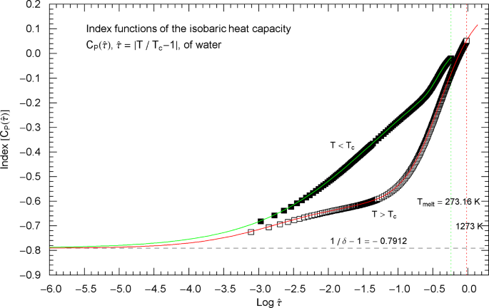
The Index function (2.7) of the low-temperature heat capacity $C_{{\text{P}}} (\tau )$ (cf. (2.5) and Table 2) is depicted in Fig. 13 as green solid curve, which represents the Log–Log slope of the subcritical branch of $C_{{\text{P}}} (\tau )$ in Fig. 12. Along the (green solid) Index curve in Fig. 13, we have indicated data points $(\tau_{i} ,{\text{Index[}}C_{{\text{P}}} (\tau_{i} )])_{i = 1,...,N}$ (filled squares) with the same abscissas as the subcritical data points $(\tau_{i} ,C_{{{\text{P}},i}} )_{i = 1,...,N}$ in Fig. 12 (also depicted by filled squares).

Outside the interval $[646.4{\text{ K}}, \, 6{47}{\text{.6 K}}]$, the Index functions in Fig. 13 do not exceed 0.7. The complement of this interval is covered by the open and filled squares in Figs. 12 and 13, representing empirical data sets of the isobaric heat capacity of water from Refs. [2, 3]. The slope of $1 - 1/\delta = 0.7912$ defining the critical power-law scaling of the isobaric heat capacity at critical pressure is only reached for temperatures extremely close to $T_{{\text{c}}} = {647}{\text{.10 K}}$, $\left| {T/T_{{\text{c}}} - 1} \right| < 10^{ - 5}$, see Fig. 13, far outside the temperature range of the empirical data of Refs. [2, 3]. Figures 14 and 15 show the high- and low-temperature heat-capacity branches and their Index functions reparametrized with reduced temperature $\hat{\tau } = \left| {t - 1} \right|$, $t = T/T_{{\text{c}}}$. The red and green straight lines in Fig. 14 depict the asymptotic power-law scaling $C_{{\rm P}} \sim A_{ \pm } \hat{\tau }^{1/\delta - 1}$.

Fig. 14

Isobaric heat capacity $C_{{\text{P}}} (\hat{\tau })$ of water at critical pressure, parametrized with reduced temperature $\hat{\tau } = \left| {T/T_{{\text{c}}} - 1} \right|$. Apart from this reparametrization, the caption of Fig. 12 is applicable. The red and green solid curves show the high- and low-temperature heat-capacity branches $C_{{\text{P}}} (\tau = 1/\hat{\tau })$ in (2.5) and Table 2, regressed from the depicted data sets, cf. Section 4. The residuals of the least-squares fits of the high- and low-temperature branches of $C_{{\text{P}}} (\hat{\tau })$ are shown in the lower panels, indicating deviations of less than one percent throughout the data range. The red and green dashed lines depicting the critical power laws $C_{{\text{P}}} (\hat{\tau } \to 0)\sim A_{ \pm } \hat{\tau }^{1/\delta - 1}$ are the asymptotes of the high- and low-temperature branches of $C_{{\text{P}}} (\hat{\tau })$

Fig. 15

Index functions of the isobaric heat capacity of water at critical pressure, parametrized with reduced temperature $\hat{\tau } = \left| {T/T_{{\text{c}}} - 1} \right|$. The red and green solid curves depict the Log–Log slope ${\text{Index[}}C_{{\text{P}}} (\tau = 1/\hat{\tau })] = - {\text{Index[}}C_{{\text{P}}} (\tau )]|_{{\tau = 1/\hat{\tau }}}$ of the high- and low-temperature branches of the heat capacity $C_{{\text{P}}} (\hat{\tau })$ in Fig. 14. The Index functions are defined in (2.7) and Table 2, subject to the substitution $\tau = 1/\hat{\tau }$ and an overall sign change as indicated. The open squares on the high-temperature ($T > T_{{\text{c}}}$) Index curve and the filled squares on the low-temperature ($T < T_{{\text{c}}}$) Index curve correspond to the heat-capacity data points in Fig. 14. The scaling exponent $1 - 1/\delta = 0.7912$ of the isobaric heat capacity is represented by the black dashed horizontal line, which is the asymptote of the Index curves. This horizontal line is also a plot of the constant Index function (Log–Log slope) of the critical power laws $A_{ \pm } \hat{\tau }^{1/\delta - 1}$ asymptotic to the high- and low-temperature branches of $C_{{\text{P}}} (\hat{\tau })$ in Fig. 14. The asymptotic power laws are depicted as parallel red and green dashed straight lines in Fig. 14

5 Hydrogen: critical isobaric heat capacity of a quantum fluid

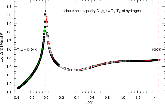
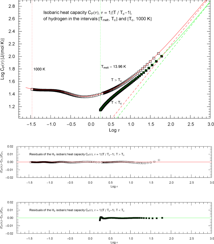
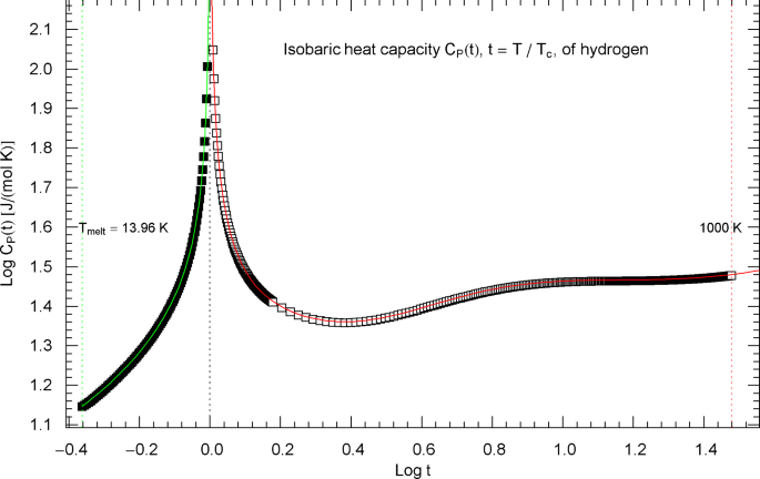
Synthetic experimental data for the isobaric heat capacity of hydrogen, cf. Refs. [2, 3], are plotted in Fig. 16, at the critical pressure of $P_{{\text{c}}} = {1}{\text{.2964 MPa}}$. Figure 16 shows a Log–Log plot of $C_{{\rm P}}$ data against reduced temperature $t = T/T_{{\text{c}}}$, from the melting point at $T_{{{\text{melt}}}} = {13}{\text{.957 K}}$ up to 32.6 K and from 33.8 K to 1000 K. The critical temperature of hydrogen is $T_{{\text{c}}} = {33}{\text{.145 K}}$, cf. Table 1.

Fig. 16

Isobaric heat capacity of hydrogen at critical pressure. Data points from Refs. [2, 3] (which are synthetic data based on a multiparameter EoS [7]), covering the low-temperature interval from the melting point $T_{{{\text{melt}}}} = {13}{\text{.957 K}}$ up to 32.6 K (92 data points, filled squares) and the high-temperature range from 33.8 K to 1000 K (398 data points, open squares). The critical temperature of hydrogen is $T_{{\text{c}}} = {33}{\text{.145 K}}$. Depicted is a Log–Log (decadic double-logarithmic) plot of the isobaric heat capacity $C_{{\text{P}}} (t)$ of hydrogen (at critical pressure $P_{{\text{c}}} = {1}{\text{.2964 MPa}}$) in reduced temperature $t = T/T_{{\text{c}}}$. The lower and upper temperature limits are indicated by the vertical green and red dotted lines. The least-squares regression is performed with the broken power-law density $C_{{\text{P}}} (\tau )$ in (5.1) (high-temperature branch, $\tau = 1/(t - 1)$, $t > 1$, red solid curve) and (5.4) (low-temperature branch, $\tau = 1/(1 - t)$, $t < 1$, green solid curve) and fitting parameters in Table 2

To model the crossover from the empirical data in Fig. 16 to the scaling regime, where $C_{{\text{P}}} \sim A_{ \pm } \left| {1 - T/T_{{\text{c}}} } \right|^{1/\delta - 1}$ with $1 - 1/\delta = 0.7912$, we parametrize the heat capacity with the scaling variable $\tau = 1/\left| {t - 1} \right|$, $t = T/T_{{\text{c}}}$. Figure 17 shows Log–Log plots of the isobaric heat-capacity data as a function of $\tau$ instead of reduced temperature. The low-temperature ($T < T_{{\text{c}}}$) data points are depicted as filled squares and the high-temperature ($T > T_{{\text{c}}}$) data as open squares, covering the same temperature range as in Fig. 16. $T_{{\text{c}}}$ in Fig. 16 is mapped to infinity in Fig. 17.

Fig. 17

Isobaric heat capacity $C_{{\rm P}} (\tau )$ of hydrogen at critical pressure, parametrized with the scaling variable $\tau = 1/\left| {T/T_{{\text{c}}} - 1} \right|$. The open and filled squares are data points from Refs. [2, 3], the same as depicted in Fig. 16. In the high-temperature regime, $T/T_{{\text{c}}} > 1$, the scaling variable is $\tau = 1/(T/T_{{\text{c}}} - 1)$, and the data points are depicted as open squares. In the low-temperature regime, $T/T_{{\text{c}}} < 1$, the scaling variable is $\tau = 1/(1 - T/T_{{\text{c}}} )$, and the data points are shown as filled squares. The red and green solid curves are the high- and low-temperature heat-capacity branches $C_{{\text{P}}} (\tau )$ in (5.1) (for $T > T_{{\text{c}}}$) and (5.4) (for $T < T_{{\text{c}}}$) regressed from the depicted data sets, cf. Table 2 and Sect. 5. The $\chi^{2}$ functional used for the regression is stated in (7.6), and the residuals of the least-squares fits of the high- and low-temperature branches are shown in the lower panels. The red and green dashed lines representing the critical power laws, cf. (5.2) and (5.5), are the asymptotes of the high- and low-temperature branches of $C_{{\text{P}}} (\tau )$ in (5.1) and (5.4). These straight lines have a Log–Log slope of $1 - 1/\delta = 0.7912$, which is the scaling exponent of the isobaric heat capacity at critical pressure

5.1 High-temperature interval from $T_{{\text{c}}}$ up to 1000 K

The data set $(\tau_{i} ,C_{{{\text{P}},i}} )$, $\tau_{i} = 1/(T_{i} /T_{{\text{c}}} - 1)$, in the high-temperature regime ($T > T_{{\text{c}}}$) comprises 398 data points in the interval between 33.8 K and 1000 K (open squares in Fig. 17, taken from Refs. [2, 3]). The least-squares fit above $T_{{\text{c}}}$ is performed with the multiply broken power law

$$C_{{\text{P}}} (\tau ) = a_{0} \tau^{{\alpha_{0} }} (1 + (\tau /b_{1} )^{{\beta_{1} /\eta_{1} }} )^{{\eta_{1} }} \frac{1}{{(1 + (\tau /b_{2} )^{{\beta_{2} /\eta_{2} }} )^{{\eta_{2} }} }}(1 + (\tau /b_{3} )^{{\beta_{3} /\eta_{3} }} )^{{\eta_{3} }} ,$$

(5.1)

with positive amplitudes $a_{0}$, $b_{k}$, positive exponents $\beta_{k}$, $\eta_{k}$, and real exponent $\alpha_{0}$ as parameters. The asymptotic limit of the broken power law (5.1) is $C_{{\text{P}}} (\tau \to \infty )\sim A_{ + } \tau^{1 - 1/\delta }$, with exponent and amplitude

$$1 - 1/\delta = \alpha_{0} + \beta_{1} - \beta_{2} + \beta_{3} ,\;A_{ + } = a_{0} b_{2}^{{\beta_{2} }} /(b_{1}^{{\beta_{1} }} b_{3}^{{\beta_{3} }} ).$$

(5.2)

The exponent $\beta_{3}$ in (5.1) is eliminated via the first identity in (5.2), using the calculated 3D Ising scaling exponent $1 - 1/\delta = 0.7912$.

The least-squares regression of $C_{{\text{P}}} (\tau )$ is explained in Appendix 1 and based on the data points $(\tau_{i} ,C_{{{\text{P}},i}} )_{i = 1,...,N}$, $N = 398$, quoted above. The fitting parameters $a_{0}$,$\alpha_{0}$,$(b_{k}^{{}} ,\beta_{k}^{{}} ,\eta_{k}^{{}} )_{k = 1,2,3}$ and the scaling amplitude $A_{ + }$ are recorded in Table 2. The regressed high-temperature branch (5.1) of the critical isobaric heat capacity $C_{{\text{P}}} (\tau )$ is depicted in Fig. 17 as red solid curve.

In Fig. 16, the isobaric heat capacity at critical pressure is parametrized with reduced temperature $t = T/T_{{\text{c}}}$. The red solid curve in this figure is the regressed high-temperature branch $C_{{\text{P}}} (\tau )$ in (5.1) with $\tau = 1/(t - 1)$, $t > 1$, substituted (shortcut $C_{{\text{P}}} (t)$). The data points depicted in Fig. 16 are the same as in Fig. 17.

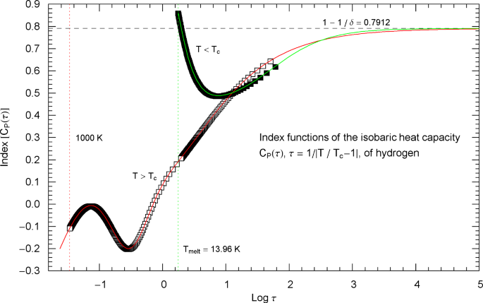
Figure 18 shows the Index function, i.e., the Log–Log slope (red solid curve) of the regressed high-temperature heat capacity $C_{{\rm P}} (\tau )$ in (5.1),

$${\text{Index[}}C_{{\text{P}}} (\tau )] = \alpha_{0} + \beta_{1} \frac{{(\tau /b_{1} )^{{\beta_{1} /\eta_{1} }} }}{{1 + (\tau /b_{1} )^{{\beta_{1} /\eta_{1} }} }} - \beta_{2} \frac{{(\tau /b_{2} )^{{\beta_{2} /\eta_{2} }} }}{{1 + (\tau /b_{2} )^{{\beta_{2} /\eta_{2} }} }} + \beta_{3} \frac{{(\tau /b_{3} )^{{\beta_{3} /\eta_{3} }} }}{{1 + (\tau /b_{3} )^{{\beta_{3} /\eta_{3} }} }}.$$

(5.3)

Fig. 18

Index functions of the critical isobaric heat capacity of hydrogen, parametrized with scaling variable $\tau = 1/\left| {T/T_{{\text{c}}} - 1} \right|$. The red and green solid curves depict the Log–Log slope ${\text{Index[}}C_{{\text{P}}} (\tau )] = {\text{d}}\log C_{{\text{P}}} (\tau )/{\text{d}}\log \tau$ of the high- and low-temperature heat-capacity branches $C_{{\text{P}}} (\tau )$, cf. Section 5. Log–Log plots of $C_{{\rm P}} (\tau )$ at critical pressure, for $T > T_{{\text{c}}}$ (cf. (5.1)) and $T < T_{{\text{c}}}$ (cf. (5.4)), are shown in Fig. 17 as red and green solid curves, respectively. The plotted Index functions ${\text{Index[}}C_{{\text{P}}} (\tau )]$ are stated in (5.3) (for $T > T_{{\text{c}}}$, red solid curve) and (5.6) (for $T < T_{{\text{c}}}$, green solid curve), with parameters in Table 2. The open squares on the (red solid) high-temperature Index curve and the filled squares on the (green solid) low-temperature Index curve correspond to the heat-capacity data points in Fig. 17. The vertical red and green dotted lines indicate the same temperature intervals as in Fig. 17. The scaling exponent $1 - 1/\delta = 0.7912$ of the heat capacity is represented by the black dashed horizontal line, which is the asymptote of the depicted Index curves (i.e., the constant $\tau \to \infty$ limit of ${\text{Index[}}C_{{\text{P}}} (\tau )]$ in (5.1) and (5.4)). This horizontal line is also a plot of the constant Index function (Log–Log slope) of the asymptotes of the high- and low-temperature branches of $C_{{\text{P}}} (\tau )$, depicted as parallel red and green dashed straight lines in Fig. 17. The latter show the asymptotic power laws (5.2) and (5.5) of the isobaric heat capacity at critical pressure

To relate Figs. 17, 18, we have plotted data points $(\tau_{i} ,{\text{Index[}}C_{{\rm P}} (\tau_{i} )])_{i = 1,...,N}$ (open squares) on the Index curve, using the abscissas $\tau_{i}$ of the high-temperature data points $(\tau_{i} ,C_{{{\text{P}},i}} )_{i = 1,...,N}$ in Fig. 17 (also indicated by open squares).

5.2 Regression of the heat capacity in the subcritical regime between $T_{{{\text{melt}}}}$ and $T_{{\text{c}}}$

The data set $(\tau_{i} ,C_{{{\text{P}},i}} )$ used for the regression of the isobaric heat capacity of hydrogen at critical pressure in the low-temperature interval $[T_{{{\text{melt}}}} ,T_{{\text{c}}} ]$ comprises 92 data points between $T_{{{\text{melt}}}} = {13}{\text{.957 K}}$ and 32.6 K (filled squares in Figs. 16 and 17, cf. Refs. [2, 3]). The least-squares fit of the low-temperature branch of $C_{{\rm P}} (\tau )$ is performed with the broken power law

$$C_{{\text{P}}} (\tau ) = a_{0} \tau^{{\alpha_{0} }} \frac{1}{{(1 + (\tau /b_{1} )^{{\beta_{1} /\eta_{1} }} )^{{\eta_{1} }} }}(1 + (\tau /b_{2} )^{{\beta_{2} /\eta_{2} }} )^{{\eta_{2} }} .$$

(5.4)

The amplitudes $a_{0}$, $b_{k}$ and exponents $\beta_{k}$, $\eta_{k}$ are positive, and the exponent $\alpha_{0}$ is real. The asymptotic power-law scaling of $C_{{\text{P}}} (\tau )$ in (5.4) reads $C_{{\text{P}}} (\tau \to \infty )\sim A_{ - } \tau^{1 - 1/\delta }$, with

$$1 - 1/\delta = \alpha_{0} - \beta_{1} + \beta_{2} ,\;A_{ - } = a_{0} b_{1}^{{\beta_{1} }} /b_{2}^{{\beta_{2} }} .$$

(5.5)

We use the scaling exponent $1 - 1/\delta = 0.7912$ to eliminate the exponent $\beta_{2}$ from $C_{{\text{P}}} (\tau )$ in (5.4) by way of the first equation in (5.5).

The least-squares regression of $C_{{\text{P}}} (\tau )$ in (5.4) is based on the subcritical data set $(\tau_{i} ,C_{{{\text{P}},i}} )_{i = 1,...,N}$, $\tau_{i} = 1/(1 - t_{i} )$, $N = 92$, indicated above. The fitting parameters $a_{0}$,$\alpha_{0}$,$(b_{k}^{{}} ,\beta_{k}^{{}} ,\eta_{k}^{{}} )_{k = 1,2}$ and the derived scaling amplitude $A_{ - }$ are listed in Table 2. The regressed $C_{{\text{P}}} (\tau )$ is shown in Fig. 17 as green solid curve. The red and green straight lines in Fig. 17 depict the asymptotic power-law scaling $C_{{\text{P}}} \sim A_{ \pm } \tau^{1 - 1/\delta }$ of the high- and low-temperature branches (5.1) and (5.4) of $C_{{\text{P}}} (\tau )$.

In Fig. 16, the regressed subcritical $C_{{\text{P}}} (\tau = 1/(1 - t))$ is plotted as a function of reduced temperature $t = T/T_{{\text{c}}} < 1$ (shortcut $C_{{\text{P}}} (t)$, green solid curve); the data points depicted in this figure are the same as in Fig. 17.

The Index function (Log–Log slope) of the low-temperature heat-capacity branch $C_{{\text{P}}} (\tau )$ in (5.4) (and Fig. 17),

$${\text{Index[}}C_{{\text{P}}} (\tau )] = \alpha_{0} - \beta_{1} \frac{{(\tau /b_{1} )^{{\beta_{1} /\eta_{1} }} }}{{1 + (\tau /b_{1} )^{{\beta_{1} /\eta_{1} }} }} + \beta_{2} \frac{{(\tau /b_{2} )^{{\beta_{2} /\eta_{2} }} }}{{1 + (\tau /b_{2} )^{{\beta_{2} /\eta_{2} }} }},$$

(5.6)

is depicted in Fig. 18 as green solid curve. On this Index curve, we have indicated data points $(\tau_{i} ,{\text{Index[}}C_{{\text{P}}} (\tau_{i} )])_{i = 1,...,N}$ (filled squares) with the same abscissas as the subcritical data points $(\tau_{i} ,C_{{{\text{P}},i}} )_{i = 1,...,N}$ in Fig. 17 (also depicted by filled squares).

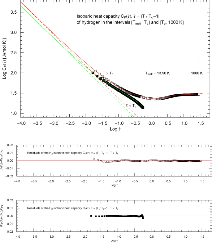
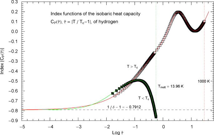
Outside the interval $[32.6{\text{ K}}, \, 33.8{\text{ K}}]$, the Index functions in Fig. 18 do not exceed 0.7, except for a section of the subcritical branch close to the melting point. The complement of this interval is covered by the open and filled squares in Figs. 17 and 18, representing empirical data sets of the critical isobaric heat capacity of hydrogen from Refs. [2, 3]. The slope of $1 - 1/\delta = 0.7912$ defining the critical power-law scaling of the isobaric heat capacity at critical pressure is only reached for temperatures extremely close to $T_{{\text{c}}} = {33}{\text{.145 K}}$, in the interval $\left| {T/T_{{\text{c}}} - 1} \right| < 10^{ - 4}$, see Fig. 18, far outside the temperature range of the empirical data of Refs. [2, 3]. Figures 19 and 20 show the high- and low-temperature heat-capacity branches and their Index functions reparametrized with reduced temperature $\hat{\tau } = \left| {t - 1} \right|$, $t = T/T_{{\text{c}}}$. The red and green straight lines in Fig. 19 depict the asymptotic power-law scaling $C_{{\text{P}}} \sim A_{ \pm } \hat{\tau }^{1/\delta - 1}$.

Fig. 19

Isobaric heat capacity $C_{{\text{P}}} (\hat{\tau })$ of hydrogen at critical pressure, parametrized with reduced temperature $\hat{\tau } = \left| {T/T_{{\text{c}}} - 1} \right|$. Apart from this reparametrization, the caption of Fig. 17 applies. The red and green solid curves show the high- and low-temperature heat-capacity branches $C_{{\text{P}}} (\tau = 1/\hat{\tau })$ in (5.1) (for $T > T_{{\text{c}}}$) and (5.4) (for $T < T_{{\text{c}}}$) regressed from the depicted data sets, cf. Section 5 and Table 2. The residuals of the least-squares fits of the high- and low-temperature branches of $C_{{\text{P}}} (\hat{\tau })$ are depicted in the lower panels, indicating deviations of less than one percent from the data points. The parallel red and green dashed straight lines depicting the critical power laws $C_{{\text{P}}} (\hat{\tau } \to 0)\sim A_{ \pm } \hat{\tau }^{1/\delta - 1}$, cf. (5.2) and (5.5), are the asymptotes of the high- and low-temperature branches of $C_{{\text{P}}} (\hat{\tau })$

Fig. 20

Index functions of the isobaric heat capacity of hydrogen at critical pressure, parametrized with reduced temperature $\hat{\tau } = \left| {T/T_{{\text{c}}} - 1} \right|$. The red and green solid curves depict the Log–Log slope ${\text{Index[}}C_{{\text{P}}} (\tau = 1/\hat{\tau })] = - {\text{Index[}}C_{{\text{P}}} (\tau )]|_{{\tau = 1/\hat{\tau }}}$ of the high- and low-temperature branches of the heat capacity $C_{{\text{P}}} (\hat{\tau })$ in Fig. 19, cf. (5.1) and (5.4). The Index functions are stated in (5.3) and (5.6) (with parameters in Table 2), subject to the substitution $\tau = 1/\hat{\tau }$ and an overall sign change as indicated. The open squares on the high-temperature ($T > T_{{\text{c}}}$) Index curve and the filled squares on the low-temperature ($T < T_{{\text{c}}}$) Index curve correspond to the heat-capacity data points in Fig. 19. The scaling exponent $1 - 1/\delta = 0.7912$ of the isobaric heat capacity at critical pressure is indicated by the black dashed horizontal line, which is the asymptote of the depicted Index curves. This horizontal line is also a plot of the constant Index function (Log–Log slope) of the critical power laws $A_{ \pm } \hat{\tau }^{1/\delta - 1}$ asymptotic to the high- and low-temperature branches of $C_{{\text{P}}} (\hat{\tau })$ in Fig. 19. The critical power laws are depicted as parallel red and green dashed straight lines in Fig. 19

6 Conclusion

The scaling theory of critical-point singularities in thermodynamic functions is experimentally amply evidenced, being largely consistent with the measured critical exponents and amplitude ratios [1, 8,9,10,11,12,13,14,15,16,17,18,19]. (There are a few exceptions, though. For instance, the scaling exponent $\beta$ of the order parameter was measured for two binary mixtures in Refs. [42, 43] and found to exceed the calculated 3D Ising exponent $\beta = 0.3264$ by about 12 percent.) The predicted power-law scaling is observable in the immediate vicinity of the critical point, leaving aside gravitational rounding effects, which set in at about $\left| {T/T_{{\text{c}}} - 1} \right| \approx 10^{ - 4}$, cf., e.g., Ref. [20].

In experimental papers, it is customary to consider a wider interval, typically $\left| {T/T_{{\text{c}}} - 1} \right| < 0.1$, and least-squares regression based on a perturbative ascending series expansion in reduced temperature, obtained by adding correction-to-scaling terms to the asymptotic power law in this extended scaling regime, cf., e.g., Refs. [11, 13, 17]. The power-law exponents are mostly identified with the calculated scaling exponents of the respective universality class, and the series coefficients are obtained by linear regression, in this way achieving consistency with renormalization-group calculations and universality.

The ideal power-law scaling interval of the isobaric heat capacity at critical pressure is particularly narrow ($\left| {T/T_{{\text{c}}} - 1} \right| < 10^{ - 5}$ for nitrogen, methane and water, and $\left| {T/T_{{\text{c}}} - 1} \right| < 10^{ - 4}$ for hydrogen), as illustrated by Index functions in Figs. 5, 10, 15 and 20. The topic of this paper was the modeling of the critical isobaric heat capacity $C_{{\text{P}}} (T,P_{{\text{c}}} )$ of fluids over a much wider temperature range far beyond the power-law scaling regime and the extended scaling regime where power-law scaling still holds with perturbative corrections. Closed-form analytic representations of the isobaric heat capacity at critical pressure were derived for nitrogen, methane, water and hydrogen, which are applicable from the melting point to the high-temperature regime where dissociation sets in.

Over this temperature range, it is not feasible to use perturbative series expansions around the critical temperature. In a safe distance from the scaling regime (quantified for the individual fluids at the beginning of each of Sects. 2, 3, 4, 5 in terms of temperature intervals), there are plenty of reliable precision data available [2, 3] for the heat capacity of the fluids studied in this paper, and we used a set of elementary closed-form distribution functions that allow for accurate nonlinear least-squares regression in the mentioned temperature range. (In the case of hydrogen, the upper temperature limit of the data range is 1000 K; dissociation into an electron–proton plasma occurs at around 5000 K.) As summarized in the caption of Table 2, the regressed distributions are structured as broken power laws factorizing as $C_{{\text{P}}} (\tau ) = a_{0} \tau^{{\alpha_{0} }} \prod\nolimits_{k = 1}^{n} {(1 + (\tau /b_{k} )^{{\beta_{k} /\left| {\eta_{k} } \right|}} )^{{ \, \eta_{k} }} }$ and are parametrized with reciprocal reduced temperature $\tau = 1/\left| {T/T_{{\text{c}}} - 1} \right|$. The fitting parameters were constrained to reproduce the asymptotic power-law scaling $\propto \left| {1 - T/T_{{\text{c}}} } \right|^{1/\delta - 1}$ with calculated scaling exponent $1 - 1/\delta$.

A systematic regression method for multiply broken power-law densities is explained in Appendix 1, and the accuracy of the least-squares fits to the experimental data sets is documented in Table 2 by the recorded value of the minimized least-squares functional of the respective fluid and, more importantly, by the residual plots in Figs. 2, 7, 12 and 17, which show the local percentage deviations of the data points from the regressed high- and low-temperature branches of the heat capacity. In Figs. 4, 9, 14 and 19, the regressed heat capacities of nitrogen, methane, water and hydrogen are depicted in reduced-temperature parametrization over several logarithmic decades, illustrating the non-perturbative analytic extension of the critical scaling regime to cover the entire temperature range from the melting point to the high-temperature regime, up to dissociation temperatures.

Appendices

Appendix 1

Nonlinear regression of multiply broken power laws subject to parameter constraints

The least-squares regression sketched in this appendix will be exemplified with the broken power law (2.1), which is parametrized with positive amplitudes $a_{0}$, $b_{k}$, positive exponents $\beta_{k}$, $\eta_{k}$ and real exponent $\alpha_{0}$. The amplitudes in (2.1) can be written as $b_{k} = 10^{{b_{10,k} }}$, with real exponent $b_{10,k}$ as fitting parameter, which is adapted to the decadic Log–Log representations of the heat capacity $C_{{\text{P}}} (\tau )$ in the figures.

When minimizing the least-squares functional (defined below), we use rescaled parameters $\hat{b}_{k}^{{}}$,$\hat{\beta }_{k}^{{}}$,$\hat{\eta }_{k}^{{}}$ related to $b_{k}^{{}}$,$\beta_{k}^{{}}$,$\eta_{k}^{{}}$ in (2.1) by

$$\hat{b}_{k}^{{}} = (10^{{b_{10,k} }} )^{{ - \beta_{k} /\eta_{k} }} ,\;\hat{\beta }_{k}^{{}} = \beta_{k} /\eta_{k} ,\;\hat{\eta }_{k}^{{}} = \eta_{k}^{{}} ,$$

(7.1)

and inversely,

$$b_{10,k} = {\text{Log}}(\hat{b}_{k}^{{ - 1/\hat{\beta }_{k} }} ),\;\beta_{k} = \hat{\beta }_{k}^{{}} \hat{\eta }_{k} ,\;\eta_{k}^{{}} = \hat{\eta }_{k}^{{}} .$$

(7.2)

(Log denotes the decadic logarithm, and $b_{k} = 10^{{b_{10,k} }}$.) The reparametrized $C_{{\text{P}}} (\tau )$ in (2.1) can be written as

$$C_{{\text{P}}} (\tau ) = a_{0} \tau^{{\alpha_{0} }} \frac{1}{{(1 + \hat{b}_{1}^{{}} \tau^{{\hat{\beta }_{1} }} )^{{ \, \hat{\eta }_{1} }} }}(1 + \hat{b}_{2}^{{}} \tau^{{\hat{\beta }_{2} }} )^{{ \, \hat{\eta }_{2} }} (1 + \hat{b}_{3}^{{}} \tau^{{\hat{\beta }_{3} }} )^{{ \, \hat{\eta }_{3} }} .$$

(7.3)

The exponents $\hat{\beta }_{k}^{{}}$,$\hat{\eta }_{k}^{{}}$ and amplitudes $\hat{b}_{k}^{{}}$ are positive like $\beta_{k}^{{}}$,$\eta_{k}^{{}}$,$b_{k}^{{}}$.

The asymptotic power-law scaling of $C_{{\text{P}}} (\tau )$ in (7.3) reads $C_{{\text{P}}} (\tau \to \infty )\sim A_{ + } \tau^{1 - 1/\delta }$, with exponent and amplitude related to the rescaled fitting parameters by

$$1 - 1/\delta = \alpha_{0} - \hat{\beta }_{1} \hat{\eta }_{1}^{{}} + \hat{\beta }_{2} \hat{\eta }_{2}^{{}} + \hat{\beta }_{3} \hat{\eta }_{3}^{{}} ,\;A_{ + } = a_{0} \hat{b}_{2}^{{\hat{\eta }_{2} }} \hat{b}_{3}^{{\hat{\eta }_{3} }} /\hat{b}_{1}^{{\hat{\eta }_{1} }} ,$$

(7.4)

which is the counterpart to Eqs. (2.2) in the new parametrization. By identifying $1 - 1/\delta$ with the calculated scaling exponent $0.7912$, the first identity in (7.4) becomes a constraint on the parameters, which can be used to eliminate the exponent $\alpha_{0}$ from $C_{{\text{P}}} (\tau )$ in (7.3), arriving at

$$C_{{\text{P}}} (\tau ) = A_{ + } \tau^{1 - 1/\delta } \frac{1}{{(1 + \hat{b}_{1}^{ - 1} \tau^{{ - \hat{\beta }_{1} }} )^{{ \, \hat{\eta }_{1} }} }}(1 + \hat{b}_{2}^{ - 1} \tau^{{ - \hat{\beta }_{2} }} )^{{ \, \hat{\eta }_{2} }} (1 + \hat{b}_{3}^{ - 1} \tau^{{ - \hat{\beta }_{3} }} )^{{ \, \hat{\eta }_{3} }} ,$$

(7.5)

with positive fitting parameters $A_{ + }$,$\hat{b}_{k}^{{}}$,$\hat{\beta }_{k}^{{}}$,$\hat{\eta }_{k}^{{}}$, $k = 1,2,3$. The exponent $1 - 1/\delta = 0.7912$ is predetermined input, and the amplitude $a_{0}$ in (7.3) is calculated from the regressed parameters via the second equation in (7.4).

The least-squares functional used for the regression reads

$$\chi ^{2} (A_{ + } ,(\hat{b}_{k} ,\hat{\beta }_{k} ,\hat{\eta }_{k} )_{{k = 1,2,3}} ) = \sum\limits_{{i = 1}}^{N} {\frac{{(C_{{\text{P}}} (\tau _{i} ) - C_{{{\text{P}},i}} )^{2} }}{{C_{{{\text{P}},i}}^{2} }}} ,$$

(7.6)

where $(\tau_{i} ,C_{{{\text{P}},i}} )_{i = 1,...,N}$ are the data points enumerated in Sect. 2.1 and $C_{{\text{P}}} (\tau )$ is the broken power law (7.5) depending on the fitting parameters $A_{ + }$,$(\hat{b}_{k}^{{}} ,\hat{\beta }_{k}^{{}} ,\hat{\eta }_{k}^{{}} )_{k = 1,2,3}$. Once these parameters are determined by minimization of the $\chi^{2}$ functional (7.6), we find the parameters $a_{0}$,$\alpha_{0}$ and $(b_{k}^{{}} ,\beta_{k}^{{}} ,\eta_{k}^{{}} )_{k = 1,2,3}$ of $C_{{\text{P}}} (\tau )$ in (2.1) by way of (7.2) and (7.4), cf. Table 2.

An efficient Mathematica® [44] routine to minimize a nonlinear $\chi^{2}$ functional such as (7.6) is FindMinimum[{chisquared[…],constraints},{initial values},MaxIterations → nmax]. The constraints are positivity constraints $\hat{b}_{k} > 0\quad \&\,\& \quad\hat{\beta }_{k}>0\quad \&\,\& \quad \hat{\eta }_{k}>0$, where the double ampersand denotes the logical AND. Alternatively, positivity constraints for the iteration can be avoided by replacing the parameters $(\hat{b}_{k}^{{}} ,\hat{\beta }_{k}^{{}} ,\hat{\eta }_{k}^{{}} )$ by $(\sqrt {\hat{b}_{k}^{2} } ,\sqrt {\hat{\beta }_{k}^{2} } ,\sqrt {\hat{\eta }_{k}^{2} } )$ in (7.5).

To find reasonably accurate initial values for the fitting parameters, which is essential in nonlinear multiparameter regression, one uses $C_{{\text{P}}} (\tau )$ in parametrization (2.1) rather than (7.5). The factors in (2.1) can be ordered by increasing amplitude, $b_{1} < b_{2} < ... < b_{n}$ (with $n = 3$ in (2.1)). In the range $\tau < < b_{k}$, the factors defined by the amplitudes $b_{k} , \, b_{k + 1} ,...,b_{n}$ are close to one and can be dropped. Therefore, an initial guess can be obtained by visually fitting the factors one by one, starting with the simple power law $a_{0} \tau^{{\alpha_{0} }}$ in (2.1) and increasing the $\tau$ range in each step by adding the respective data points and the respective factor. The amplitudes $b_{k}$ are the break points between the power-law segments (which are straight line segments in Log–Log plots) and the exponents $\eta_{k}$ determine the extent (curvature) of the transitional regions.

References

A. Pelissetto, E. Vicari, Phys. Rep. 368, 549 (2002). https://doi-org../10.1016/S0370-1573(02)00219-3
E.W. Lemmon, I.H. Bell, M.L. Huber, M.O. McLinden, NIST Standard Reference Database 23, Reference Fluid Thermodynamic and Transport Properties-REFPROP, Version 10.0, 2018. https://www.nist.gov/srd/refprop
E.W. Lemmon, M.O. McLinden, D.G. Friend, in P.J. Linstrom, W.G. Mallard (Eds.), NIST Chemistry WebBook, NIST Standard Reference Database 69 (2021). https://webbook.nist.gov/chemistry/fluid/
R. Span, E.W. Lemmon, R.T. Jacobsen, W. Wagner, A. Yokozeki, J. Phys. Chem. Ref. Data 29, 1361 (2000). https://doi-org../10.1063/1.1349047
U. Setzmann, W. Wagner, J. Phys. Chem. Ref. Data 20, 1061 (1991). https://doi-org../10.1063/1.555898
W. Wagner, A. Pruß, J. Phys. Chem. Ref. Data 31, 387 (2002). https://doi-org../10.1063/1.1461829
J.W. Leachman, R.T. Jacobsen, S.G. Penoncello, E.W. Lemmon, J. Phys. Chem. Ref. Data 38, 721 (2009). https://doi-org../10.1063/1.3160306
H. Güttinger, D.S. Cannell, Phys. Rev. A 24, 3188 (1981). https://doi-org../10.1103/PhysRevA.24.3188
A. Haupt, J. Straub, Phys. Rev. E 59, 1795 (1999). https://doi-org../10.1103/PhysRevE.59.1795
D.S. Cannell, Phys. Rev. A 12, 225 (1975). https://doi-org../10.1103/PhysRevA.12.225
U. Närger, D.A. Balzarini, Phys. Rev. B 39, 9330 (1989). https://doi-org../10.1103/PhysRevB.39.9330
L.M. Radzhabova, G.V. Stepanov, I.M. Abdulagatov, K.A. Shakhbanov, J. Supercrit. Fluids 63, 115 (2012). https://doi-org../10.1016/j.supflu.2011.11.017
A. Kostrowicka Wyczalkowska, Kh.S. Abdulkadirova, M.A. Anisimov, J.V. Sengers, J. Chem. Phys. 113, 4985 (2000). https://doi-org../10.1063/1.1289244
J.A. Lipa, J.A. Nissen, D.A. Stricker, D.R. Swanson, T.C.P. Chui, Phys. Rev. B 68, 174518 (2003). https://doi-org../10.1103/PhysRevB.68.174518
J.R. de Bruyn, D.A. Balzarini, Phys. Rev. B 39, 9243 (1989). https://doi-org../10.1103/PhysRevB.39.9243
J.A. Lipa, C. Edwards, M.J. Buckingham, Phys. Rev. A 15, 778 (1977). https://doi-org../10.1103/PhysRevA.15.778
M.W. Pestak, M.H.W. Chan, Phys. Rev. B 30, 274 (1984). https://doi-org../10.1103/PhysRevB.30.274
P. Losada-Pérez, C.A. Cerdeiriña, J. Thoen, J. Chem. Thermodyn. 128, 356 (2019). https://doi-org../10.1016/j.jct.2018.08.035
P. Losada-Pérez, C.S.P. Tripathi, J. Leys, C. Glorieux, J. Thoen, J. Chem. Phys. 134, 044505 (2011). https://doi-org../10.1063/1.3535567
M.R. Moldover, J.V. Sengers, R.W. Gammon, R.J. Hocken, Rev. Mod. Phys. 51, 79 (1979). https://doi-org../10.1103/RevModPhys.51.79
M. Barmatz, I. Hahn, J.A. Lipa, R.V. Duncan, Rev. Mod. Phys. 79, 1 (2007). https://doi-org../10.1103/RevModPhys.79.1
A. Oprisan, J.J. Hegseth, G.M. Smith, C. Lecoutre, Y. Garrabos, D.A. Beysens, Phys. Rev. E 84, 021202 (2011). https://doi-org../10.1103/PhysRevE.84.021202
A. Oprisan, S.A. Oprisan, Y. Garrabos, C. Lecoutre-Chabot, D. Beysens, Eur. Phys. J. Plus 136, 523 (2021). https://doi-org../10.1140/epjp/s13360-021-01531-8
R.B. Griffiths, J.C. Wheeler, Phys. Rev. A 2, 1047 (1970). https://doi-org../10.1103/PhysRevA.2.1047
J. Stephenson, J. Chem. Phys. 54, 895 (1971). https://doi-org../10.1063/1.1675016
A. Callegari, A. Magazzù, A. Gambassi, G. Volpe, Eur. Phys. J. Plus 136, 213 (2021). https://doi-org../10.1140/epjp/s13360-020-01020-4
S. El-Showk, M.F. Paulos, D. Poland, S. Rychkov, D. Simmons-Duffin, A. Vichi, J. Stat. Phys. 157, 869 (2014). https://doi-org../10.1007/s10955-014-1042-7
R. Tomaschitz, Physica A 541, 123188 (2020). https://doi-org../10.1016/j.physa.2019.123188
R. Tomaschitz, Eur. Phys. J. Plus 136, 629 (2021). https://doi-org../10.1140/epjp/s13360-021-01542-5
X. Gabaix, Q. J. Econ. 114, 739 (1999). https://doi-org../10.1162/003355399556133
X. Gabaix, Annu. Rev. Econ. 1, 255 (2009). https://doi-org../10.1146/annurev.economics.050708.142940
A. Clauset, C.R. Shalizi, M.E.J. Newman, SIAM Rev. 51, 661 (2009). https://doi-org../10.1137/070710111
E. Puppin, Eur. Phys. J. Plus 135, 420 (2020). https://doi-org../10.1140/epjp/s13360-020-00398-5
M.E.J. Newman, Contemp. Phys. 46, 323 (2005). https://doi-org../10.1080/00107510500052444
J.B. McDonald, Econometrica 52, 647 (1984). https://doi-org../10.2307/1913469
J.B. McDonald, Y.J. Xu, J. Econ. 66, 133 (1995). https://doi-org../10.1016/0304-4076(94)01612-4
R. Tomaschitz, Physica A 611, 128421 (2023). https://doi-org../10.1016/j.physa.2022.128421
J.S. Kouvel, M.E. Fisher, Phys. Rev. 136, A1626 (1964). https://doi-org../10.1103/PhysRev.136.A1626
J.V. Sengers, J.G. Shanks, J. Stat. Phys. 137, 857 (2009). https://doi-org../10.1007/s10955-009-9840-z
R. Tomaschitz, J. Supercrit. Fluids 181, 105491 (2022). https://doi-org../10.1016/j.supflu.2021.105491
R. Tomaschitz, Int. J. Thermophys. 43, 130 (2022). https://doi-org../10.1007/s10765-022-03034-9
N. Fameli, D.A. Balzarini, Phys. Rev. B 75, 064203 (2007). https://doi-org../10.1103/PhysRevB.75.064203
P. Venkatesu, J. Chem. Phys. 123, 024902 (2005). https://doi-org../10.1063/1.1953576
Wolfram Research, Inc., Mathematica,® Version 13.1, Champaign, IL, (2022). https://www.wolfram.com/mathematica/
Author information
Authors and Affiliations
Corresponding author