Modeling electrical resistivity and particle fluxes with multiply broken power-law distributions

Multiply broken power-law densities are introduced to model empirical data sets extending over several logarithmic decades. Two examples demonstrating the wide range of applicability of these distributions are discussed. First, the temperature dependence of the electrical resistivity of metals (Cu, Au, Cr, Al, W, Fe, Ni) is inferred by nonlinear least-squares regression covering the solid phase up to the melting point. The regressed broken power laws are compared with high- and low-temperature scaling predictions obtained from electron–phonon and electron–electron scattering. In the intermediate temperature range, inflection points arise in Log–Log plots of the electrical resistivity, unaccounted for by the Bloch–Grüneisen theory. In the second example, the energy evolution of cosmic-ray electron and positron fluxes is analyzed in terms of multiply broken and exponentially cut power-law densities, based on recently obtained number counts. Index functions quantifying the spectral variation and survival functions (complementary cumulative distributions) of the particle and energy fluxes are calculated from the regressed densities.

Graphic abstract

The aim is to demonstrate the efficiency of multiply broken power-law distributions in high-precision modeling of empirical data. Two very different examples will be analyzed to that effect, the temperature evolution of the electrical resistivity of metals and the energy evolution of particle fluxes, the latter specified by cosmic-ray electron and positron spectra.

The main part of this paper deals with the mentioned applications, but we will also sketch the general formalism of power-law densities [1,2,3,4,5,6], their logarithmic representation and Index functions, their complementary cumulative distribution functions (CCDFs), as well as Weibull [7,8,9,10,11,12,13] and lognormal [14,15,16,17,18,19] cutoffs. The nonlinear least-squares regression of multiply broken and exponentially cut power-law densities will be discussed as well.

Multiply broken power-laws are introduced in Sect. 2.1, composed of power-law segments with smooth transitions at the break points, which are particularly suitable for the modeling of data sets extending over several logarithmic decades [20, 21]. In Sect. 2.2, we study cutoff factors (which are asymptotically Weibull exponentials or lognormals) for multiply broken power-law distributions and derive their Index functions. In Sect. 22,23,24,25] are performed. We study the Index functions of the total and intrinsic resistivities and compare the regressed temperature evolution with the linear temperature scaling of the Drude resistivity/conductivity theory in the high-temperature regime and with the $T^{2}$ and $T^{5}$ low-temperature scaling predicted by electron–electron and electron–phonon scattering, cf. e.g., [26, 27]. (The intrinsic resistivity is obtained by subtraction of the constant residual resistivity caused by impurity scattering.) In most cases, power-law scaling laws with integer exponents do not give accurate descriptions of the high- and low-temperature limits of the empirical resistivity data, not even approximately.

In Sect. 4, the modeling of cosmic-ray particle fluxes with multiply broken power-law densities is studied. The recently observed electron and positron fluxes [28,29,30] can accurately be described by power-law distributions with two spectral breaks and an exponential cutoff. At first sight, the decaying flux densities seem to admit simple power-law tails over an extended energy range, but the actual structure of these spectra is more varied, as illustrated by their Index functions. The tails of the electronic/positronic survival functions also largely deviate from simple power-law and lognormal distributions. The entropy of the electron/positron fluxes is calculated from the regressed broken power laws. Section 5 contains the conclusions.

In Appendix A, we summarize some elementary facts about power laws, lognormals and Weibull (stretched and compressed exponential) cutoffs in double-logarithmic representation, as well as their Index functionals representing the Log–Log slope of analytic distributions inferred by least-squares regression.

Broken power laws with smooth transitions

Broken power laws are defined as finite products [31, 32]

with positive amplitudes $A_{0}$, $b_{k}$, positive exponents $\beta_{k}$, real exponent $\beta_{0}$ and positive or negative exponents $\eta_{k}$. It is also understood that the factors are ordered by increasing amplitude $b_{k} < b_{k + 1}$. The distribution $p(x)$ consists of $n + 1$ approximate power-law segments, $\propto x^{{\beta_{0} }}$,$x^{{\beta_{0} + \beta_{1} {\text{sign}}(\eta_{1} )}}$,…,$x^{{\beta_{0} + \sum\nolimits_{k = 1}^{n} {\beta_{k} {\text{sign}}(\eta_{k} )} }}$, in the intervals $x < < b_{1}$, $b_{1} < < x < < b_{2} , \ldots ,b_{n} < < x$, respectively. The amplitudes $b_{k}$ define the break points between the power-law segments and the exponents $\eta_{k}$ determine the extent of the transitional regions; $\left| {\eta_{k} } \right| < < 1$ implies a narrow transitional interval with a sudden change of slope at $b_{k}$. Power laws in Log–Log plots show as approximately straight segments, and the exponents $\eta_{k}$ determine the curvature of the transitions and the width of the transitional region between the power-law segments.

The Feller–Pareto (or generalized beta) distribution is a special case of (2.1), obtained by putting $n = 1$ in the product, cf. Ref. [33]. This distribution consists of two power-law components, $\propto x^{{\beta_{0} }}$ for $x < < b_{1}$ and $\propto x^{{\beta_{0} + \beta_{1} {\text{sign}}(\eta_{1} )}}$ for $x > > b_{1}$, and a smooth transition around the break point $b_{1}$ and has been used to model income and wealth distributions [34, 35].

A practical way to quantify deviations from power-law scaling is provided by Index functions, occasionally employed in economic modeling, cf. e.g., Refs. [4, 5, 8, 34]. The Index function of a multiply broken power-law distribution (2.1) reads

and gives the Log–Log slope of the distribution, cf. Appendix A for an elementary discussion of Index functions. In Sect. 3, we will employ Index functions to test power-law scaling predictions of the electrical resistivity of metals, arriving at the conclusion that the power-law scaling suggested by ab initio calculations based on various scattering mechanisms is not particularly accurate when compared with precision measurements of high-purity samples.

The introduction of multiply broken power-law distributions is motivated by the need to model ever bigger data sets stretching over several logarithmic decades, and standard textbook distributions [33] are insufficient to cope with that. A possible way to describe extended data sets is to use joint distributions, that is, to partition the data range into intervals and to use different standard distributions in each interval, joining them at the interval boundaries, cf. e.g., Refs. [36, 37]. Smoothness (differentiability) conditions at the interval boundaries then result in analytically rather complex distributions. The multiply broken power-law distributions (2.1) composed of structurally identical factors and the additive Index functions (2.2) offer a more uniform and technically simpler way to model extended data sets.

As pointed out above, the distribution (2.1) has power-law asymptotics, $p(x)\sim {\text{const}}{. }x^{{\beta_{0} + \sum\nolimits_{k = 1}^{n} {\beta_{k} {\text{sign}}(\eta_{k} )} }}$, for $x > > b_{n}$. In the next section, we will discuss multiply broken power laws admitting exponential or lognormal decay, by adding a cutoff factor to the product (2.1), which will be used in Sect. 4 to model electronic and positronic particle fluxes.

Cutoff factors of multiply broken power laws

Weibull decay

A Weibull cutoff of the broken power law $p(x)$ in (2.1) is obtained by adding the cutoff factor $W(x) = \exp ( - (x/d)^{\delta } )$ to the product, with positive $\delta$, $d$ (and $d > b_{n}$, see after (2.1)). The exponent $\delta$ defines stretched ($0 < \delta < 1$) or compressed ($\delta > 1$) exponential decay. The Index function of $W(x)$ is found as $I_{W} (x) = xW^{\prime}(x)/W(x) = - \delta (x/d)^{ \, \delta }$, to be added to the series in (2.2). That is, the Index function of the exponentially cut power law $p(x)W(x)$ is $I_{pW} (x) = I_{p} (x) + I_{W} (x)$.

Weibull cutoff with adaptable crossover

We generalize the above Weibull cutoff by defining, in analogy to the factors of the broken power law (2.1),

which gives the standard Weibull cutoff in the limit $b \to 0$, cf. Section 2.2.1. The second summand in the exponential is just a normalization factor, so that $W(0) = 1$. The amplitudes $b$,$d$ ($d > b_{n}$, cf. (2.1)) and exponents $\delta$, $\eta$ are positive fitting parameters. $W(x)$ is monotonously decaying, the crossover to the asymptotic regime depends on the exponent $\eta$, and the parameter $b$ can be determined from the asymptotic amplitude factor $\exp ((b/d)^{\delta } )$.

The Index function of $W(x)$ in (2.3) reads

and the Index function of the exponentially cut density $p(x)W(x)$ is $I_{pW} (x) = I_{p} (x) + I_{W} (x)$, where $p(x)$ is the multiply broken power law (2.1) and $I_{p} (x)$ and $I_{W} (x)$ are the Index functions in (2.2) and (2.4).

Lognormal decay

A lognormal cutoff of the multiply broken power law $p(x)$ in (2.1) is generated by adding the factor

where $b$,$\beta$,$\delta$ are positive parameters and $\eta$ is positive or negative. This cutoff is obtained by substituting $(1 + (x/b)^{\beta /\left| \eta \right|} )$ for $x$ in the lognormal $x^{ \, \eta - \delta \log x}$, cf. Appendix A, according to the pattern (2.1). Asymptotically, $w(x)\sim \tilde{A}x^{{ \, \tilde{\eta } - \tilde{\delta }\log x}}$, with constants $\tilde{A}$, $\tilde{\eta }$, $\tilde{\delta }$ depending on the fitting parameters $b$,$\beta$,$\delta$,$\eta$. Also, $w(0) = 1$. If the exponent $\eta$ is negative, $w(x)$ is monotonously decaying. If $\eta$ is positive, $w(x)$ attains a maximum before the decay sets in. The Index function of $w(x)$ in (2.5) reads

The Index function of the lognormally cut power law $p(x)w(x)$, cf. (2.1) and (2.5), is obtained by adding the Index functions in (2.2) and (2.6), $I_{pw} (x) = I_{p} (x) + I_{w} (x)$. Lognormal cutoffs have been used to model city-size and firm-size tail distributions, cf. e.g., Refs. [16,17,18,19] and references therein.

Analyticity of multiply broken power laws

The broken power-law density $p(x)$ in (2.1) is analytic along the positive real axis but not at $x = 0$, unless integer exponents are used, because of a branch cut along the negative real axis. In some applications, analyticity at $x = 0$ is essential, for instance, when an ascending series expansion is required [38]. To make $p(x)$ analytic at $x = 0$, we replace $x \to a_{k} + x$ in each factor, where the $a_{k}$ are positive fitting parameters, and also normalize each factor in (2.1) to one at $x = 0$ except the first (with exponent $\beta_{0}$). In this way, $p(x)$ in (2.1) is transformed into

The positive constants $a_{k}$, like the amplitudes $b_{k}$ and the exponents $\beta_{k}$,$\eta_{k}$, are to be determined by least-squares regression. The shift $a_{0}$ can be put to zero from the outset if $\beta_{0}$ is a positive integer, and the same holds true for $a_{k}$ if the exponent $\beta_{k} /\left| {\eta_{k} } \right|$ is integer, cf. after (2.1), but the exponents are usually real fitting parameters. The Index function $I_{p} (x) = xp^{\prime}(x)/p(x)$ of density $p(x)$ in (2.7) reads

obtained from (2.2) by shifting $x \to a_{k} + x$ and adding a factor $x/(a_{k} + x)$ to each summand.

The Weibull cutoff factor defined in Sect. 2.2.1 can also be made analytic at $x = 0$ (if $\delta$ is non-integer) by shifting $x \to a + x$, $a > 0$, and normalizing, $W(x) = \exp (a/d)^{\delta } \exp [ - ((a + x)/d)^{\delta } ]$, so that $W(0) = 1$. The Index function of $W(x)$ is obtained from $I_{W} (x)$ in Sect. 2.2.1 by shifting $x \to a + x$ and adding the factor $x/(a + x)$, so that $I_{W} (x) = - \delta ((a + x)/d)^{\delta } x/(a + x)$.

The adaptable Weibull cutoff (2.3) can be made analytic in the same way, by replacing $x \to a + x$ and subsequent normalization to $W(0) = 1$,

The Index function of $W(x)$ reads, cf. (2.4),

Analogously, the lognormal cutoff $w(x)$ in (2.5) becomes analytic at $x = 0$ via the shift $x \to a + x$ and normalization to $w(0) = 1$,

and admits the Index function

obtained from (2.6) by shifting $x \to a + x$ and adding the factor $x/(a + x)$, as in (2.10).

The resistivity data used [22,23,24,25] cover several logarithmic decades in temperature, from the low-temperature regime up to the melting point. The classical Drude model of electrical resistivity predicts a linear temperature slope at high temperature. At low temperature, a $T^{5}$ dependence is predicted by the Bloch–Grüneisen theory based on electron–phonon scattering, and a quadratic temperature dependence is suggested by electron–electron scattering, cf. the reviews [26, 27]. This refers to the ideal solid, discounting impurities. The actual low-temperature limit of the resistivity is constant (temperature independent) due to electron–impurity scattering.

We split the electrical resistivity into two components, $\rho (T) = \rho_{{{\text{res}}}} + \rho_{{{\text{int}}}} (T)$, where $\rho_{{{\text{res}}}}$ is the constant residual resistivity due to impurities. $\rho_{{{\text{int}}}} (T)$ denotes the intrinsic temperature-dependent resistivity, modeled as a multiply broken power-law density (2.1). The parameters defining $\rho_{{{\text{int}}}} (T)$ are obtained by least-square regression. In the examples below, we will study the temperature evolution of the electrical resistivity of copper, gold, chromium, aluminum, tungsten, iron and nickel.

The Index function $I_{\rho } (T)$ defining the Log–Log slope of the total resistivity $\rho (T) = \rho_{{{\text{res}}}} + \rho_{{{\text{int}}}} (T)$ reads, cf. Section 2.1,

where the Index $I_{{\rho {\text{int}}}} (T)$ defines the slope of the intrinsic resistivity $\rho_{{{\text{int}}}} (T)$. Thus, if the resistivity is dominated by electron–electron scattering in some low-temperature interval, this implies the Log–Log slope $I_{{\rho {\text{int}}}} (T) \approx 2$. If electron–phonon scattering is dominant at low temperature, $I_{{\rho {\text{int}}}} (T) \approx 5$. In the high-temperature regime, the Drude model predicts $I_{{\rho {\text{int}}}} (T) \approx I_{\rho } (T) \approx 1$.

Copper and gold

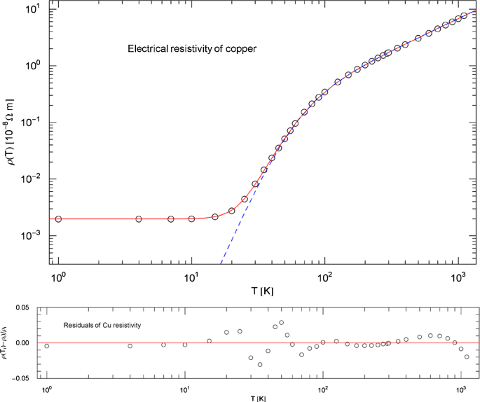
For the total electrical resistivity $\rho (T) = \rho_{{{\text{res}}}} + \rho_{{{\text{int}}}} (T)$ of copper, we use the recommended data set of Ref. [22], which assumes 99.999% pure copper (annealed), and the data are corrected for thermal expansion. The least-squares regression in Fig. 1 is performed with a broken power law for the intrinsic resistivity, cf. (2.1) (with $n = 1$),

Electrical resistivity of copper. Data points from Ref. [22]. The red solid curve depicts the total resistivity $\rho (T) = \rho_{{{\text{res}}}} + \rho_{{{\text{int}}}} (T)$, where $\rho_{{{\text{int}}}} (T)$ (blue dashed curve) is the intrinsic resistivity (modeled as broken power-law density (3.2)) and $\rho_{{{\text{res}}}}$ the constant residual resistivity due to impurities. The fitting and goodness-of-fit parameters are listed in Table 1. $\rho_{{{\text{int}}}} (T)$ is obtained by subtracting $\rho_{{{\text{res}}}}$ (a fitting parameter) from the regressed total resistivity $\rho (T)$. The temperature range extends up to the melting point at 1357.8 K. Residuals of the least-squares fit of $\rho (T)$ are depicted in the lower panel

Full size image

This is the simplest case of the broken power law (2.1), admitting only one break point $b_{1}$, cf. Section 2.1, which is actually a standard distribution, a generalized beta distribution of the second kind, cf. Refs. [33,34,35]. The amplitudes and (positive) exponents are fitting parameters, as well as the residual resistivity $\rho_{{{\text{res}}}}$, cf. Table 1 where also the goodness-of-fit parameters are listed. The least-squares fit $\rho (T)$ (red solid curve) and the intrinsic resistivity $\rho_{{\text{int}}} (T)$ (dashed blue curve) of copper are depicted in Fig. 1. The Index function of the intrinsic resistivity $\rho_{{\text{int}}} (T)$ in (3.2) reads, cf. (2.2),

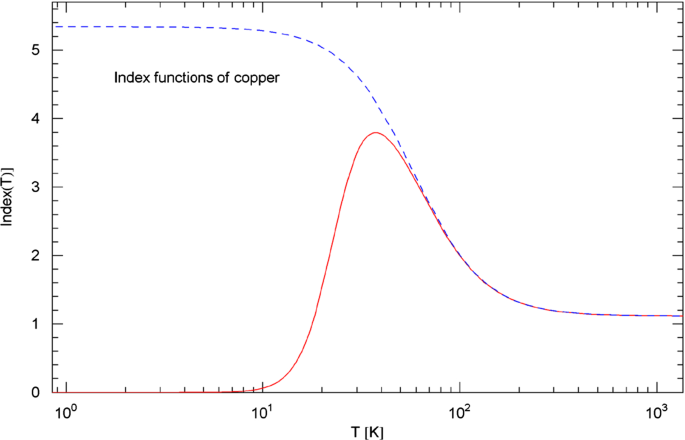
which is depicted in Fig. 2 together with the Index $I_{\rho } (T)$ of the total resistivity, cf. (3.1).

Index functions of copper. The red solid curve depicts the Index function $I_{\rho } (T)$ of the total resistivity in (3.1), calculated with the residual and intrinsic resistivities $\rho_{{{\text{res}}}}$ and $\rho_{{{\text{int}}}} (T)$ extracted from the least-squares fit in Fig. 1. The blue dashed curve shows the Index function $I_{{\rho {\text{int}}}} (T)$ of the intrinsic resistivity, cf. (3.3). These Index functions represent the Log–Log slope of the resistivity curves in Fig. 1. At high temperature, the slope is nearly linear, with Index close to one (classical temperature scaling of resistivity). At low temperature, the Index of the intrinsic resistivity is close to five, indicating dominant electron–phonon scattering which predicts a $T^{5}$ resistivity scaling

Full size image

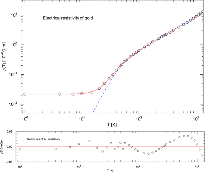
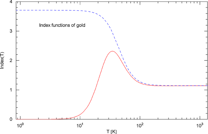
Figures 3 and 4 show the resistivities and the Index functions of gold (99.999% purity, annealed, data points [22] corrected for thermal expansion). The intrinsic resistivity $\rho_{{\text{int}}} (T)$ and the least-squares fit of the total resistivity $\rho (T) = \rho_{{{\text{res}}}} + \rho_{{{\text{int}}}} (T)$ are plotted in Fig. 3, based on the broken power law (3.2), like in the case of copper. The fitting parameters are stated in Table 1. The Index functions (3.1) and (3.3) of the total and intrinsic resistivities of gold are depicted in Fig. 4.

Electrical resistivity of gold. Data points from Ref. [22]. The caption of Fig. 1 applies. The red solid curve depicts the least-squares fit of the total resistivity $\rho (T) = \rho_{{{\text{res}}}} + \rho_{{{\text{int}}}} (T)$, cf. (3.2) and Table 1, with residual resistivity $\rho_{{{\text{res}}}}$ and intrinsic resistivity $\rho_{{{\text{int}}}} (T)$ (blue dashed curve). The fitting parameters are listed in Table 1. The temperature range is cut off at the melting point (1337.3 K). Residuals of the least-squares fit are depicted in the lower panel

Full size image

Index functions of gold. The caption of Fig. 2 applies. Depicted are the Index functions of the total electrical resistivity $I_{\rho } (T)$ (red solid curve) and intrinsic resistivity $I_{{\rho {\text{int}}}} (T)$ (blue dashed curve) in (3.1) and (3.3), obtained from the least-squares fit in Fig. 3. At high temperature, the temperature scaling of the resistivity of gold is steeper than linear. The Index of the intrinsic resistivity is lower than four over the full temperature range of the solid phase; a $T^{5}$ scaling of the intrinsic resistivity at low temperature predicted by the Bloch–Grüneisen theory based on electron–phonon scattering is not visible

Full size image

As pointed out in Sect. 2.1 and Appendix A, the Index functions quantify the slope of the Log–Log resistivity curves. That is, a tangent to the resistivity curves represents a power law $\propto T^{\alpha }$, where the exponent $\alpha$ is the slope of the tangent line (in Log–Log coordinates) given by the Index function. In this section, we will use Index functions to check power-law scaling predictions of resistivity derived from electron–phonon scattering (Bloch–Grüneisen theory, suggesting a $T^{5}$ power law for the intrinsic resistivity at low temperature) and electron–electron scattering (generating a low-temperature $T^{2}$ contribution to the intrinsic resistivity). Which of these power laws is dominant also depends on the amplitudes. The Bloch–Grüneisen formula for the intrinsic resistivity of metals, which interpolates between the $T^{5}$ scaling and the linear high-temperature scaling predicted by the classical Drude model of resistivity, is reviewed in Refs. [26, 27], including the derivation from linearized transport theory; for the latter, see also Refs. [39, 40] and references therein. Here, we will focus on the $T^{2}$ and $T^{5}$ scaling predictions by comparing with empirical data, and find that they are somewhat idealized.

The Index functions of gold and copper in Figs. 2 and 4 have a similar shape. At high temperature, the Index is only slightly above one ($\beta_{0} - \beta_{1} = 1.12$ for copper and $\beta_{0} - \beta_{1} = 1.15$ for gold, cf. (3.2), (3.3) and Table 1), so that the linear temperature scaling of the Drude model is approximately realized. In the low temperature regime, the Index $I_{{\rho {\text{int}}}} (T)$ of the intrinsic resistivity of copper (blue dashed curve in Fig. 2) is noticeably above five ($\beta_{0} = 5.34$, cf. Table 1). For gold, the Index stays below four ($\beta_{0} = 3.71$), cf. Figure 4, so that a $T^{5}$ low-temperature scaling of the intrinsic resistivity predicted by the Bloch–Grüneisen theory is not evidenced; a $T^{2}$ slope suggested by electron–electron scattering is not visible either. Temperature intervals where simple power-law scaling $\propto T^{\alpha }$ applies are indicated by nearly constant horizontal segments of the Index curves with ordinate $\approx \alpha$, cf. Appendix A. Power-law scaling in the high- and low-temperature regimes is clearly shown by the Index curves of the intrinsic resistivity in Figs. 2 and 4, albeit with exponents deviating from the scaling predictions of scattering theory.

Chromium

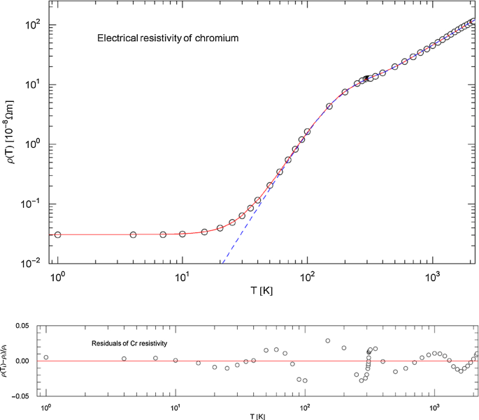
Figures 5 and 6 depict the least-squares fit of the resistivity and the Index function of chromium, based on recommended data points in Ref. [23] (99.98% purity, data corrected for thermal expansion). The $\chi^{2}$ fit of the total resistivity $\rho (T) = \rho_{{{\text{res}}}} + \rho_{{{\text{int}}}} (T)$ is performed with the broken power-law density (2.1) (with $n = 2$),

Electrical resistivity of chromium. Data points from Ref. [23]. The least-squares fit of the total resistivity $\rho (T) = \rho_{{{\text{res}}}} + \rho_{{{\text{int}}}} (T)$ (red solid curve) is performed with the broken power law $\rho_{{{\text{int}}}} (T)$ (blue dashed curve) in (3.4). $\rho_{{{\text{res}}}}$ and $\rho_{{{\text{int}}}} (T)$ denote the residual and intrinsic resistivities. The fitting and goodness-of-fit parameters are stated in Table 1. A Log–Log inflection point (black filled circle) emerges at the Néel temperature of 308 K. The temperature range is cut off at the melting point (2180 K)

Full size image

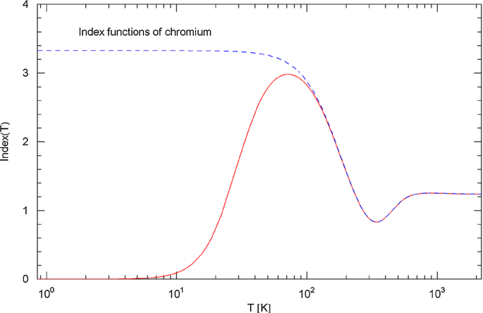
Index functions of chromium. Depicted is the Index (Log–Log slope) of the total and intrinsic resistivities in Fig. 5. The red solid curve shows the Index $I_{\rho } (T)$ of the total resistivity $\rho (T)$, cf. (3.1). The blue dashed curve is the Index $I_{{\rho {\text{int}}}} (T)$ of the intrinsic resistivity $\rho_{{{\text{int}}}} (T)$, cf. (3.5). As in the previous examples, the Index at high temperature is larger than one, in contrast to the linear scaling of the Drude resistivity model. The low-temperature scaling exponent $\beta_{0}$ of the intrinsic resistivity, cf. Table 1, is somewhat larger than three; the quadratic scaling due to electron–electron scattering and the $T^{5}$ scaling predicted by electron–phonon scattering is not evidenced. At the Néel temperature of 308 K, the Index function has a local minimum

Full size image

representing the intrinsic resistivity. (All exponents and amplitudes in (3.4) are positive.).

The Index function thereof reads, cf. (2.2),

The Index $I_{\rho } (T)$ of the total resistivity of chromium, cf. (3.1), and the Index $I_{{\rho {\text{int}}}} (T)$ of the intrinsic resistivity in (3.5) are depicted in Fig. 6. The approximately constant segments of the Index curves in Fig. 6 indicate power-law scaling. At high temperature close to the melting point, the scaling exponent is significantly above one, $\beta_{0} - \beta_{1} + \beta_{2} = 1.24$, cf. (3.4), (3.5) and Table 1. The low-temperature limit of the Index of the intrinsic resistivity in Fig. 6 indicates a power law with exponent $\beta_{0} = 3.33$, quite different from the scaling predictions based on electron–electron and electron–phonon scattering. The Néel transition of chromium happens at 308 K, manifested by a dent in the Index curve. Power-law scaling is shown by the intrinsic Index curves in Fig. 6 below 10 K and above $10^{3} {\text{K}}$, but not with the integer exponents of the Bloch–Grüneisen theory.

Aluminum and tungsten

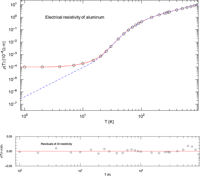
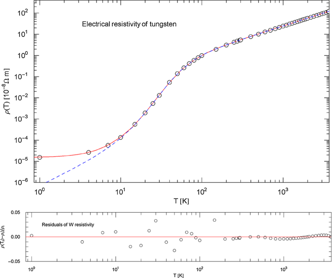
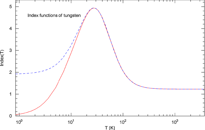
Figures 7, 8, 9, 10 depict the total and intrinsic resistivities of aluminum and tungsten and their Index functions. The recommended aluminum data set is from Ref. [24], and the tungsten data are from Ref. [25]. The data sets refer to 99.99% purity and are corrected for thermal expansion. The least-squares fits of the total resistivity $\rho (T) = \rho_{{{\text{res}}}} + \rho_{{{\text{int}}}} (T)$ in Figs. 7 and 9 are performed with the broken power law, cf. (2.1),

Electrical resistivity of aluminum. Data points from Ref. [24]. The $\chi^{2}$ fit is performed with the total resistivity $\rho (T) = \rho_{{{\text{res}}}} + \rho_{{{\text{int}}}} (T)$ (red solid curve). The intrinsic resistivity $\rho_{{{\text{int}}}} (T)$ (blue dashed curve) is the broken power law (3.6). The fitting parameters are stated in Table 2. The temperature range extends up to the melting point at 933.47 K. Residuals are depicted in the lower panel

Full size image

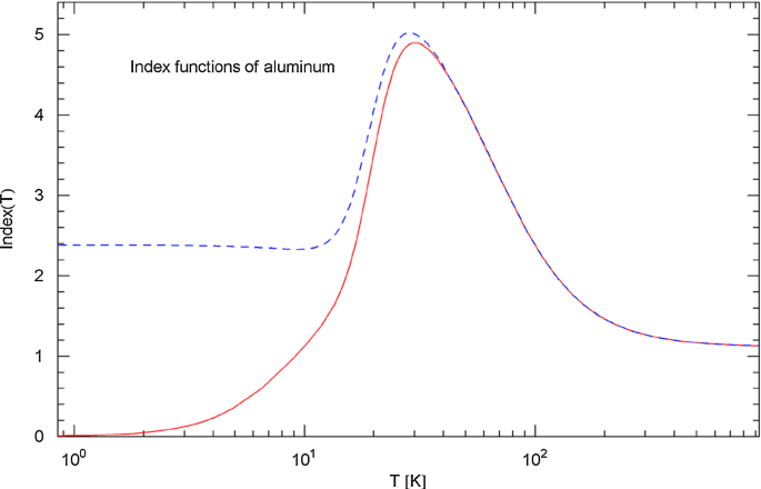
Index functions of aluminum. Depicted are the Index function $I_{\rho } (T)$ of the total resistivity (red solid curve, cf. (3.1)), which is the Log–Log slope of the regressed resistivity $\rho (T)$ in Fig. 7, and the Index of the intrinsic resistivity $I_{{\rho {\text{int}}}} (T)$ (blue dashed curve), cf. (3.7). At high temperature, the Index is slightly larger than one, fairly close to the classical linear temperature scaling of resistivity. At low temperature, the Index of the intrinsic resistivity is close to two, suggesting that electron–electron scattering is dominant. The Index of five predicted by electron–phonon scattering is only reached at the maximum of the Index curves at around 30 K, where the Log–Log plot of the resistivity in Fig. 7 has an inflection point

Full size image

Electrical resistivity of tungsten. Data points from Ref. [25]. The red solid curve shows the $\chi^{2}$ fit of the total resistivity, $\rho (T) = \rho_{{{\text{res}}}} + \rho_{{{\text{int}}}} (T)$. The intrinsic resistivity $\rho_{{{\text{int}}}} (T)$ (blue dashed curve) is the broken power law (3.6), obtained by subtracting the residual resistivity $\rho_{{{\text{res}}}}$ (a fitting parameter, cf. Table 2) from the regressed $\rho (T)$. The temperature range is cut off at the melting point (3687 K)

Full size image

Index functions of tungsten. The Index $I_{\rho } (T)$ of the total resistivity is depicted as red solid curve, cf. (3.1), and the Index $I_{{\rho {\text{int}}}} (T)$ of the intrinsic resistivity in (3.7) as blue dashed curve, calculated with the fitting parameters in Table 2. These Index curves depict the Log–Log slope of the resistivities in Fig. 9. At high temperature, the Index is close to one, as predicted by the classical Drude model of resistivity. At low temperature, the Index of the intrinsic resistivity is close to two, reflecting the quadratic temperature scaling due to electron–electron scattering. At around 30 K, the Index is close to five, in a narrow interval like in the case of aluminum, cf. Fig. 8; a $T^{5}$ slope of the resistivity indicates dominant electron–phonon scattering

Full size image

with positive amplitudes and exponents. The fitting and goodness-of-fit parameters are recorded in Table 2. The Index function of the intrinsic resistivity (3.6) reads, cf. (2.2),

The Index functions $I_{{\rho {\text{int}}}} (T)$ and $I_{\rho } (T)$ (cf. (3.1)) of aluminum and tungsten are depicted in Figs. 8 and 10. The high-temperature Index shows power-law scaling of the resistivity with exponent $\beta_{0} + \beta_{1} - \beta_{2} = 1.12$ for Al and $\beta_{0} + \beta_{1} - \beta_{2} = 1.23$ for W, cf. (3.6), (3.7) and Table 2. At low temperature, the Index of the intrinsic resistivity is $\beta_{0} = 2.38$ for Al and $\beta_{0} = 1.91$ for W, cf. Table 2), suggesting dominant electron–electron scattering (indicated by a quadratic temperature dependence of the intrinsic resistivity). A slope exponent close to five (due to electron–phonon scattering according to the Bloch theory) is reached in a narrow temperature range around 30 K, for aluminum and tungsten alike. Thus, in the case of Al and W, the predictions of scattering theory are at least qualitatively met, cf. Figures 8 and  10: at low temperature, the intrinsic resistivity is mostly generated by electron–electron scattering, followed by a crossover to the $T^{5}$ scaling stemming from electron–phonon scattering and a subsequent crossover to the linear classical scaling regime close to the melting point.

Iron and nickel

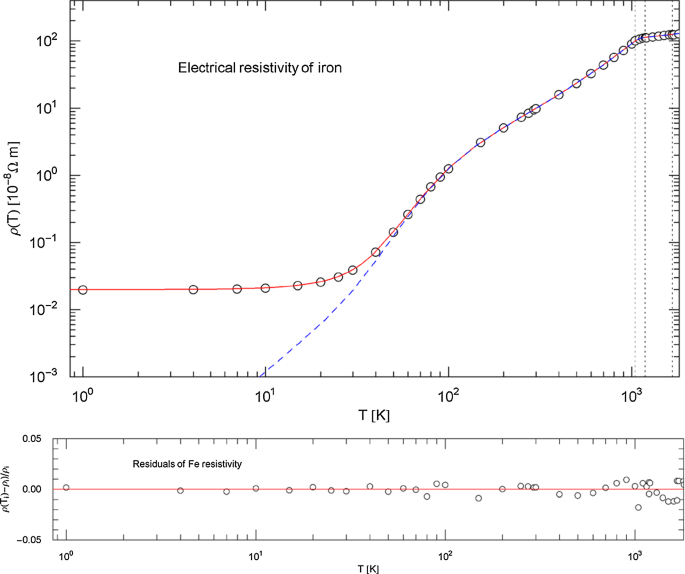
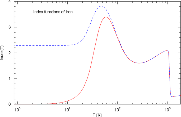
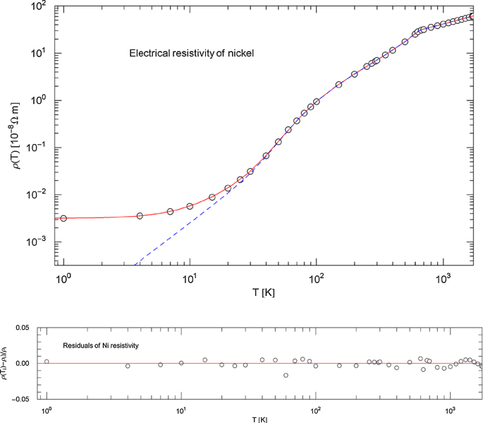
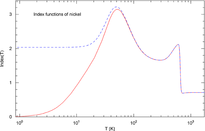
Figures 11, 12, 13 and 14 show the total and intrinsic resistivities of iron and nickel, based on data sets in Ref. [23] (99.99% purity, corrected for thermal expansion), and the corresponding Index functions $I_{\rho } (T)$ and $I_{{\rho {\text{int}}}} (T)$. By the way, the temperature range shown in the figures is cut off at the melting point of the respective metal, where a discontinuity emerges in the resistivity, cf. Refs. [22,23,24,25].

Electrical resistivity of iron. Data points from Ref. [23]. Depicted is the least-squares fit of the total resistivity $\rho (T) = \rho_{{{\text{res}}}} + \rho_{{{\text{int}}}} (T)$ (red solid curve), with constant residual resistivity $\rho_{{{\text{res}}}}$. The intrinsic resistivity $\rho_{{{\text{int}}}} (T)$ (blue dashed curve) is the multiply broken power law (3.8). The fitting and goodness-of-fit parameters are stated in Table 2. The temperature range extends up to the melting point at 1811 K. The vertical dotted lines indicate the Curie temperature at 1043 K and the $\alpha \to \gamma$ transition at 1185 K and $\gamma \to \delta$ transition at 1667 K

Full size image

Index functions of iron. The Index $I_{\rho } (T)$ of the total resistivity $\rho (T) = \rho_{{{\text{res}}}} + \rho_{{{\text{int}}}} (T)$, cf. (3.1), is depicted as red solid curve, based on the least-squares fit in Fig. 11 with parameters in Table 2. The Index function $I_{{\rho {\text{int}}}} (T)$ of the intrinsic resistivity, cf. (3.9), is shown as blue dashed curve. A steep drop of the Index, effectively a discontinuity, occurs at the Curie temperature of 1043 K. Above this temperature, the Index is nearly constant up to the melting point (1811 K) and substantially smaller than one, largely deviating from the classical linear temperature scaling of the Drude resistivity model. At low temperature, the Index of the intrinsic resistivity is rather close to two, suggesting dominant electron–electron scattering. The maximum of the Index curve is attained at around 50 K and is smaller than four. A $T^{5}$ slope of the intrinsic resistivity due to electron–phonon scattering is not reached within the temperature range of the solid phase. Local extrema of the Index curves indicate inflection points of the resistivity curves in Fig. 11

Full size image

Electrical resistivity of nickel. Data points from Ref. [23]. The red solid curve depicts the least-squares fit of the total resistivity, $\rho (T) = \rho_{{{\text{res}}}} + \rho_{{{\text{int}}}} (T)$. The intrinsic resistivity $\rho_{{{\text{int}}}} (T)$ (blue dashed curve) is modeled with the broken power law (3.8), as in the case of iron in Fig. 11. The fitting parameters are recorded in Table 2; the residual resistivity $\rho_{{{\text{res}}}}$ due to impurities is also treated as free parameter in the least-squares fit of $\rho (T)$. The temperature range is cut off at the melting point (1728 K). Residuals of the $\chi^{2}$ fit are shown in the lower panel

Full size image

Index functions of nickel. Depicted is the Index $I_{\rho } (T)$ of the total resistivity in (3.1) (red solid curve) and the Index $I_{{\rho {\text{int}}}} (T)$ of the intrinsic resistivity in (3.9) (blue dashed curve), with parameters in Table 2. The Index functions show the Log–Log slope of the regressed resistivity curves in Fig. 13. The Curie temperature of 627 K is marked by a sudden drop of the Index. The high-temperature Index is smaller than one, in contrast to the linear temperature scaling of resistivity in the classical Drude model. The low-temperature Index of the intrinsic resistivity is close to two, caused by electron–electron scattering. Like in the case of iron, the maximum of the Index functions is attained at around 50 K and barely exceeding three, so that the low-temperature scaling predicted by the Bloch–Grüneisen theory is not evidenced. The local minima and maxima of the Index curves correspond to inflection points of the resistivity curves in Fig. 13

Full size image

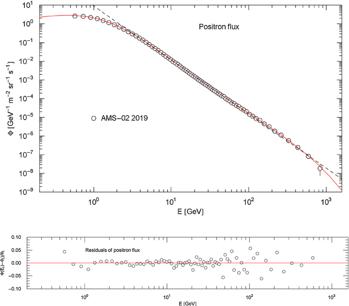
Flux density of cosmic-ray positrons. Data points from AMS-02 [28]. The red solid curve is a least-squares fit of the particle flux density $\Phi (E)$ in (4.1), which is a broken power law with two spectral breaks and exponential cutoff, cf. after (4.1). The fitting parameters are recorded in Table 3 and the goodness-of-fit parameters in Table 4. The black dashed straight line is a power-law fit $\Phi (E) \propto E^{{ - 2.89}}$ in the interval 2−830 GeV, cf. Table 5. Residuals of the regressed $\Phi (E)$ are depicted in the lower panel

Full size image

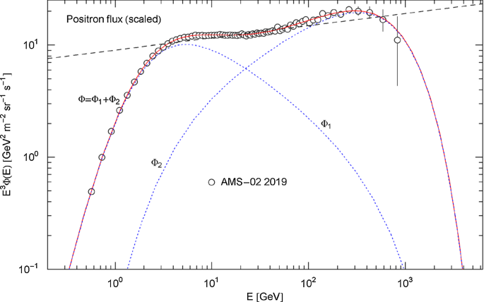
Rescaled positronic flux density and additive decomposition thereof. Data points as in Fig. 15. The scale factor E³has the effect that the rescaled low- and high-energy flux points are of similar magnitude, in contrast to Fig. 15. The red solid curve depicts the rescaled flux density $E^{3} \Phi (E)$ in (4.1), and the black dashed line is the rescaled power-law fit in Fig. 15. This rescaling demonstrates, without resorting to goodness-of-fit parameters, that a power-law fit is not suitable even in the intermediate energy range. The blue dotted curves show the additive decomposition of the flux density into two spectral peaks, cf. (4.2)

Full size image

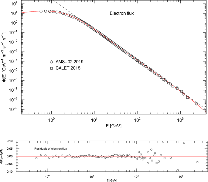
Flux density of cosmic-ray electrons. Data points from AMS-02 (circles) [29] and CALET (squares) [30]. (The original data points from the CALET detector refer to the combined electron and positron flux. The depicted electronic data points (squares) were obtained by subtraction of the regressed positronic flux density in Fig. 15.) The red solid curve is the regressed electronic flux density $\Phi (E)$, cf. (4.1) and Tables 3 and 4. The black dashed straight line is a power-law fit $\Phi (E) \propto E^{{ - 3.20}}$in the range 4–2400 GeV, with parameters in Table 5 Residuals of the twice broken and exponentially cut power-law density $\Phi (E)$ in (4.1) and Table 3 are depicted in the lower panel

Full size image

In the case of iron, the depicted temperature range covers the Curie temperature at 1043 K and also the solid phase transitions $\alpha \to \gamma$ at 1185 K and $\gamma \to \delta$ at 1667 K (indicated by dotted vertical lines in Fig. 11). The Curie temperature of nickel is 627 K. The least-squares fits of the total resistivity $\rho (T) = \rho_{{{\text{res}}}} + \rho_{{{\text{int}}}} (T)$ in Figs. 11 and 13 are performed with the multiply broken power law (2.1) ($n = 4$),

with positive exponents, whose Index function reads, cf. (2.2),

The fitting and goodness-of-fit parameters of the iron and nickel resistivities are recorded in Table 2. The Index functions $I_{\rho } (T)$ and $I_{{\rho {\text{int}}}} (T)$ of the total and intrinsic resistivities are depicted in Figs. 12 and 14. Above the Curie temperature, marked by a sudden drop of the Index, effectively a discontinuity, the resistivities exhibit power-law scaling up to the melting point, but with an exponent substantially below the classical linear scaling, $\beta_{0} + \beta_{1} - \beta_{2} + \beta_{3} - \beta_{4} = 0.37$ for iron and $\beta_{0} + \beta_{1} - \beta_{2} + \beta_{3} - \beta_{4} = 0.71$ for nickel, cf. (3.8), (3.9) and Table 2. At low temperature, the Index of the intrinsic resistivity indicates power-law scaling with exponent $\beta_{0} = 2.29$ for iron and $\beta_{0} = 2.04$ for nickel, cf. Table 2, qualitatively consistent with electron–electron scattering. A $T^{5}$ slope that can be associated with electron–phonon scattering is not reached anywhere in both cases; the maximum of the Index functions is located at around 50 K and stays below four. The local extrema of the Index curves in Figs. 12 and 14 correspond to inflection points of the Log–Log plots of the resistivities in Figs. 11 and 13, cf. Appendix A. The Index functions of these ferromagnets are similarly structured, and clearly discernible from the dia- and paramagnetic materials in Sects. 3.1 and 3.3 and also from the antiferromagnetic chromium in Sect. 3.2.

Particle fluxes as multiply broken and exponentially cut power laws

Wideband spectra of cosmic-ray fluxes provide examples of multiply broken power-law distributions with Weibull cutoff. In this section, we discuss recently measured electron and positron fluxes [28,29,30]. The flux density of cosmic-ray positrons or electrons is defined as $\Phi (E) = {\text{d}}N(E)/{\text{d}}E$, where ${\text{d}}N(E)$ is the differential number count (particles per second per square meter per steradian) parametrized with the (kinetic) particle energy. The units used for the flux density are $1/{\text{(GeV s m}}^{{2}} {\text{ sr)}}$. $\Phi (E)$ is modeled as a twice broken and exponentially cut power-law density, cf. Section 2.2.1 and Ref. [41],

with positive amplitudes $A_{0}$, $b_{1} < < b_{2} < < d_{0}$, and positive exponents $\beta_{0}$, $\beta_{1,2}$, $\eta_{1,2}$, $\delta_{0}$. The particle flux density $\Phi (E)$ is composed of three approximate power-law segments $\propto E^{{\beta_{0} }}$, $E^{{\beta_{0} - \beta_{1} }}$, $E^{{\beta_{0} - \beta_{1} + \beta_{2} }}$ in the intervals $E < < b_{1}$, $b_{1} < < E < < b_{2}$, $b_{2} < < E < < d_{0}$ and a subsequent exponential Weibull cutoff for $E > > d_{0}$, cf. Sections 2.1 and 2.2.1.

When performing a nonlinear $\chi^{2}$ fit of the multi-parameter distribution $\Phi (E)$, a good initial guess of the fitting parameters in (4.1) is indispensable (when minimizing the $\chi^{2}$ functional, cf. the caption of Table 1). The product representation of the distribution offers a systematic way to find an initial guess. First, we note that the factor defined by amplitude $b_{1}$ does not significantly change the density in the range $E < < b_{1}$, and the factor defined by $b_{2}$ does not affect the density in the range $E < < b_{2}$. The cutoff factor does not affect the density in the range $E < < d_{0}$. (This is also the reason to use normalization factors in (2.7), (2.9) and (2.11).) Therefore, one can obtain an initial guess by visually fitting the factors one by one, increasing the energy range in each step (by adding the respective data points), which is further facilitated by the fact that the above-mentioned power-law segments appear as approximate straight lines in Log–Log plots, cf. Appendix A. Analogous reasoning applies for the least-squares fits of the electrical resistivity in Sect. 3.

The regression of the positron and electron fluxes shown in Figs. 15, 16, 17, 18 is performed with density $\Phi (E)$ in (4.1), where we specify the exponents as $\eta_{2} = \delta_{0} = 1$, since the currently available data points in Refs. [28,29,30] (used in the fits) do not suffice to determine these exponents. Previous experiments measuring the positron [42,43,44,45,46,47,48] and electron [44, 45, 47, 49,50,51,52,53,54,55,56] fluxes or the combined fluxes have substantially larger error bars or are even incompatible with the recent AMS-02 [28, 29] and CALET [30] data sets.

Since $\eta_{2} = 1$ from the outset, the flux density (4.1) can be split into two components, $\Phi (E) = \Phi_{1} (E) + \Phi_{2} (E)$,

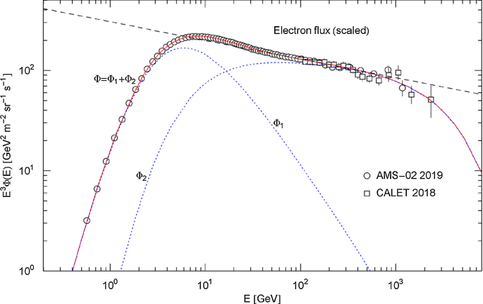
More generally, by specifying the exponent $\eta_{2}$ in (4.1) as integer $n$, the flux density can be decomposed into $n + 1$ additive components (radiation peaks). Such additive decompositions are empirically not really verifiable, though often attempted, cf. e.g., Refs. [28, 29] in this context, especially if the presumed peaks of the measured density are as closely spaced and substantially overlapping as in the case of the positron and electron distributions studied here. We have indicated the decomposition (4.2) in Figs. 16 and 18, but will otherwise refrain from speculating about the origins of these peaks, the more so as there could several be hidden in the measured densities. Instead, in Sect. 4.2, we will interpret $\Phi (E)$ as the flux density of a stationary ultra-relativistic plasma, by employing an effective partition function.

Figures 15 and 17 show the regressed particle flux densities (4.1), with fitting and goodness-of-fit parameters in Tables 3 and 4. At first sight, a simple power-law tail fit $\Phi (E) \propto E^{ - \alpha }$ seems to be the obvious choice, given that power laws appear as straight lines in Log–Log plots. These power-law fits are indicated as black dashed lines in Figs. 15 and 17, with parameters listed in Table 5 (including the energy interval in which the fit is performed). Figures 16 and 18 show the same least-squares fits of the flux densities as Figs. 15 and 17, but rescaled by a factor of $E^{3}$, so that the rescaled flux values have roughly the same magnitude at low and high energy. Also depicted in Figures 16 and 18 are the rescaled power-law fits (dashed black lines) in the intermediate energy range. In this representation, it becomes evident that simple power-law fits are not an accurate representation of the data points, not even at intermediate energies. The spectral breaks are clearly visible in the rescaled plots in Figures 16 and 18. To obtain an initial guess for the least-squares fit of $\Phi (E)$, one uses the $E^{3}$-scaled data points, proceeds as outlined after (4.1), and subsequently rescales with $E^{ - 3}$.

Rescaled electron flux and additive decomposition thereof. Data points as in Fig. 17. The red solid curve depicts the rescaled flux density $E^{3} \Phi (E)$, cf. (4.1), obtained from the least-squares fit of $\Phi (E)$ in Fig. 17 and Tables 3 and 4. The black dashed line is the rescaled power-law fit in Fig. 17 and Table 5. The blue dotted curves show the $E^{3}$ scaled decomposition of the electron flux in (4.2). The positronic counterpart is depicted in Fig. 16

Full size image

Thermodynamic variables of stationary non-equilibrium fluxes

To define the entropy functional of the empirical flux density $\Phi (E)$ in (4.1) (with δ₀ = 1), we employ an effective spectral number density, ${\text{d}}\rho (E)/{\text{d}}E = sE^{2} {\text{e}}^{ - \beta E - h(E)} /(2\pi^{2} (\hbar c)^{3} )$, where $h(E)$ is a spectral function to be determined from the regressed flux density. If $h(E)$ is constant, $h(E) = \alpha$, then ${\text{d}}\rho (E)/{\text{d}}E$ is the number density of an ultra-relativistic classical electron or positron gas in equilibrium, where $\beta = 1/(k_{{\text{B}}} T)$, $\alpha$ is the fugacity parameter and $s = 2$ the spin degeneracy. The spectral density ${\text{d}}\rho (E)/{\text{d}}E$ is angular-integrated and related to the flux $\Phi (E)$ (in steradian) by ${\text{d}}\rho (E)/{\text{d}}E = 4\pi {\text{ sr }}\Phi (E)/c$. Accordingly, the temperature variable can be identified with the cutoff exponent $d_{0}$ in (4.1), $k_{{\text{B}}} T = d_{0}$, cf. Table 3, and the spectral function $h(E)$ reads

with spin multiplicity $s = 2$. The amplitude $A_{0}$ has the dimension indicated in Table 3, so that the argument of the log is dimensionless.

When deriving thermodynamic variables, it is convenient to write the spectral density ${\text{d}}\rho (E)/{\text{d}}E$ in slightly more general form [8, 41],

with two dimensionless parameters $\alpha_{0}$ and $\alpha_{h}$. The specific number and energy densities of particles above a threshold energy $E$ then read

where the derivatives and the spectral density ${\text{d}}\rho (E)$ are taken at $\alpha_{0} = 0$ and $\alpha_{h} = 1$, so that ${\text{d}}\rho (E) = (4\pi {\text{ sr}}/c{) }\Phi (E){\text{d}}E$ as stated above. The partition function can be identified by way of (4.5), $\log Z(E;\beta ,\alpha_{0} ,\alpha_{h} ) = V\int_{E}^{\infty } {{\text{d}}\rho } (E)$, with ${\text{d}}\rho (E)$ in (4.4), so that $N = \log Z(E;\beta ,0,1)$.

The entropy of particles above the threshold energy $E$ is found as

taken at $\alpha_{0} = 0$ and $\alpha_{h} = 1$. Hence, $S/k_{{\text{B}}} = N + \beta U + N_{h}$, where, cf. (4.5) and (4.6),

The spectral representation of entropy thus reads $S = k_{{\text{B}}} V\int_{E}^{\infty } {(1 + \beta E + h(E)){\text{d}}\rho } (E)$, with $h(E)$ in (4.3). ${\text{d}}\rho (E)$ is the spectral number density in (4.4) (with $\alpha_{0} = 0$, $\alpha_{h} = 1$). The equilibrium entropy is recovered with a constant spectral function $h(E) = \alpha$, where the fugacity parameter $\alpha$ is related to the chemical potential by $\mu = - \alpha /\beta$. We use the spectral function $h(E)$ in (4.3) (with parameters in Table 3) and $E = 0$ as lower integration boundary (since the electronic rest mass is negligible at GeV energies), to estimate the specific energy density of the electron flux as $S/(k_{{\text{B}}} V) = 2.25 \times 10^{ - 4}$. The entropy density of the positron flux is one order lower, $S/(k_{{\text{B}}} V) = 2.52 \times 10^{ - 5}$.

In the case of a stretched or compressed Weibull cutoff in (4.1), one can replace βE in spectral density (4.4) by $\hat\beta_0E+ \hat\beta_1(E/d_0)^{\delta_0}$ and put $\hat\beta_0=0$ and $\hat\beta_1=1$ after differentiation, proceeding analogously as in (4.5)–(4.8). In the spectral representation of entropy, the term βE is then replaced by $(E/d_0)^{\delta_0}$.

Electronic/positronic survival functions extracted from wideband spectra

Normalization of the regressed particle flux density $\Phi (E)$ in (4.1) gives the probability density $p(E) = \Phi (E)/\int_{0}^{\infty } {\Phi (E){\text{d}}E}$. The survival function (complementary cumulative distribution function, CCDF) is then obtained as

where $\int_{E}^{\infty } {\Phi (E){\text{d}}E}$ counts the number of detected particles (per unit time per unit area per steradian) with energy exceeding the threshold energy $E$, and $S(E)$ is the probability that a detected particle has a kinetic energy exceeding $E$.

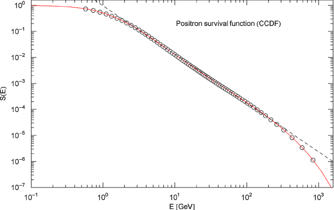
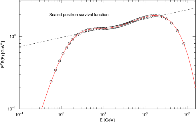
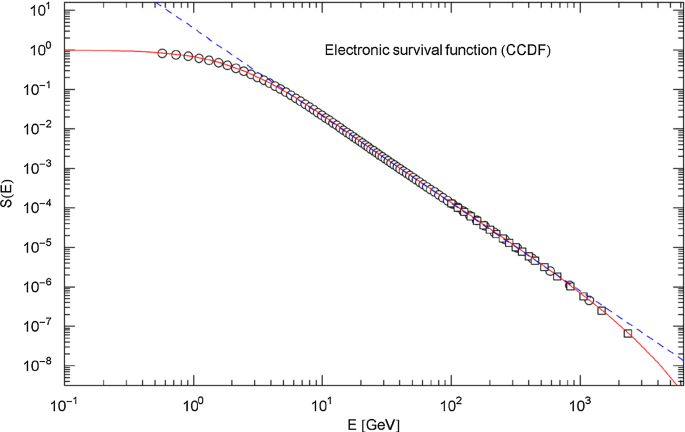
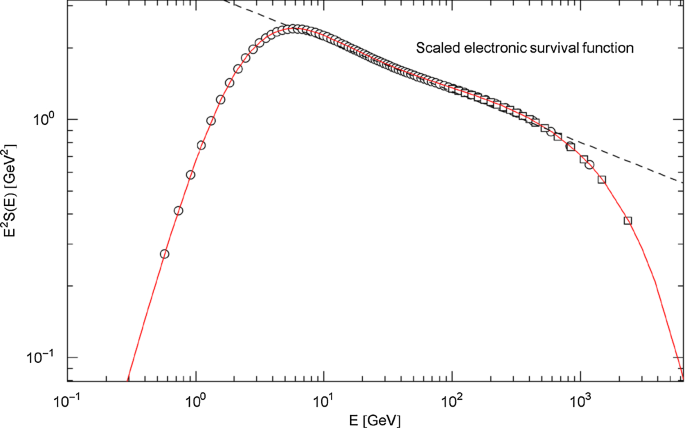
Figures 19, 20, 21 and 22 show the survival functions $S(E)$ of the positron and electron fluxes, calculated from the regressed flux densities $\Phi (E)$ in (4.1) and Table 3, together with power-law approximations $S(E) \approx A \, E^{ - \beta }$ in the intermediate energy range (black dashed straight lines). The parameters of the power-law fits in Figs. 19 and 21 and the energy range in which they are performed are listed in Table 6. Figures 20 and 22 show the $E^{2}$-rescaled survival functions and their power-law approximations, the latter illustrating the limits of linear regression.

Positronic survival function. The red solid curve shows the survival function $S(E)$ in (4.9) (normalized complementary cumulative distribution), calculated with the regressed positronic flux density in (4.1) and Table 3. The indicated data points $(E_{i} ,S(E_{i} ))$ (circles) are located at the same energies as the flux points in Fig. 15. The black dashed line is a power-law fit $S(E) \propto E^{ - 1.87}$ to the data points in the 2 GeV − 330 GeV range, cf. Table 6

Full size image

Scaled positron survival function. The caption of Fig. 19 applies, except that the survival function $S(E)$ in (4.9) (red solid curve) has been rescaled by a factor of $E^{2}$. The black dashed line is the $E^{2}$ scaled power-law fit in Fig. 19 and Table 6, which is evidently a poor fit, even in the intermediate energy range

Full size image

Electron survival function. The survival function $S(E)$ in (4.9) (red solid curve) is calculated with the flux density (4.1) and parameters in Table 3. The depicted data points $(E_{i} ,S(E_{i} ))$ (circles, rectangles) refer to the energies $E_{i}$ of the measured flux points in Fig. 17. The blue dashed line is a power-law fit $S(E) \propto E^{ - 2.21}$ to the data points in the 3−1500 GeV interval, cf. Table 6

Full size image

Scaled electron survival function. The red solid curve depicts the $E^{2}$ scaled survival function $S(E)$, cf. (4.9) and Fig. 21, based on the flux density (4.1) with fitting parameters in Table 3. The black dashed line is the $E^{2}$ scaled power-law fit in Fig. 21 and Table 6, approximating the survival function in the intermediate energy range

Full size image

Index functions of cosmic-ray electron and positron fluxes

The Index function defining the Log–Log slope of the particle flux density $\Phi (E)$ in (4.1) reads, cf. (2.2) and Sect. 2.2.1,

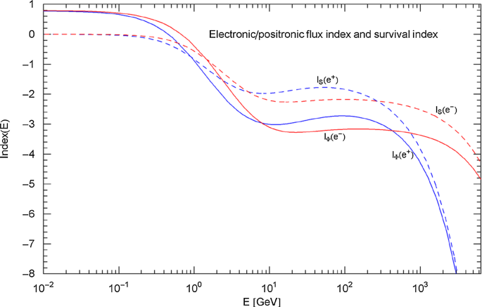
Figure 23 shows plots of the Index functions of the regressed positronic and electronic flux densities $\Phi (E)$ with parameters in Table 3. Also shown in Fig. 23 are the Indices of the associated electronic and positronic survival functions $S(E)$ in (4.9),

Index functions of the electronic/positronic flux density $\Phi (E)$ and survival function $S(E)$. The red (electronic) and blue (positronic) solid curves depict the Index function $I_{\Phi } (E)$ (cf. (4.10)) of the particle flux density $\Phi (E)$ in (4.1). The Index $I_{\Phi } (E)$ represents the Log–Log slope of the flux densities $\Phi (E)$ in Figs. 15 and 17, cf. Section 2.1. The red/blue dashed curves show the Index $I_{S} (E)$ in (4.11), i.e., the Log–Log slope of the electronic/positronic survival function $S(E)$ in (4.9) and Figs. 19 and 21. In contrast, the Index functions of the power-law fits depicted as dashed straight lines in Figs. 15, 17, 19 and 21 are constant and would appear here as horizontal lines (with power-law exponent as ordinate). The minima and maxima of the depicted Index curves indicate the location of the inflection points of the particle flux densities (in Figs. 15 and 17) and survival functions in Figs. 19 and 21, cf. Appendix A

Full size image

The Index (i.e., Log–Log slope) of the flux densities $\Phi (E)$ in Figs. 15 and 17 substantially varies, in contrast to the constant slopes of the power-law fits (black dotted straight lines in Figs. 15 and 17), and the same holds true for the Index of the survival functions $S(E)$ in Figs. 19 and 21. Local minima and maxima of the Index functions in Fig. 23 indicate Log–Log inflection points of the positronic/electronic $\Phi (E)$ (in Figs. 15 and 17) and $S(E)$ (in Figs. 19 and 21), cf. Appendix A.

Complementary cumulative energy flux

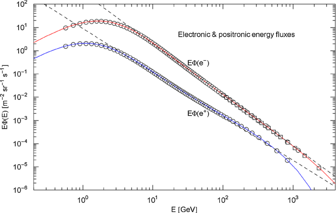
The electronic and positronic energy flux densities $E\Phi (E)$ are plotted in Fig. 24, based on the regressed particle (number) flux density $\Phi (E)$ in (4.1) with parameters in Table 3. The power-law fits in Figs. 15 and 17 (with parameters in Table 5) are also indicated in Fig. 24, rescaled with energy (black dashed straight lines).

Energy flux densities. The red/blue solid curves show the electronic/positronic energy flux density $E\Phi (E)$, cf. Section 4.5, defined by the regressed particle flux density $\Phi (E)$ in (4.1) with fitting parameters in Table 3. The depicted data points $(E_{i} ,E_{i} \Phi (E_{i} ))$ (circles, squares) are located at the same energies as the particle flux data in Figs. 15 and 17. The dashed straight lines indicate the $E$ scaled power-law fits in Figs. 15 and 17, $E\Phi (E) \propto E^{ - 1.89}$ for positrons and $E\Phi (E) \propto E^{ - 2.20}$ for electrons

Full size image

The cumulative energy flux (per unit time per unit area per steradian) of particles with kinetic energy up to a threshold energy $E$ is calculated as $U(E) = \int_{0}^{E} {E\Phi (E){\text{d}}E}$. The complementary cumulative energy flux $U_{{{\text{CC}}}} (E)$ reads accordingly

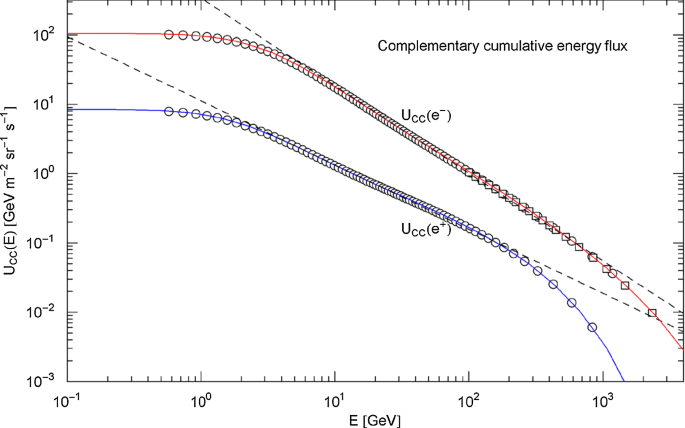
so that $U_{{{\text{CC}}}} (0)$ is the total kinetic particle energy (per second per square meter per steradian) absorbed by the detector. The specific energy density is $(4\pi {\text{ sr}}/c)U_{{{\text{CC}}}} (0)$, the rest mass in the electronic/positronic dispersion relation being negligible in the GeV range; the factor of $4\pi$ stems from the solid-angle integration. This gives a specific energy density of ${3}{\text{.52}} \times 10^{ - 7} {\text{ GeV/m}}^{{3}}$ for positrons, one order smaller than the electronic energy density of ${4}{\text{.39}} \times 10^{ - 6} {\text{ GeV/m}}^{{3}}$. The energy density $U/V$ in (4.6) is related to the complementary cumulative energy flux by $U/V = (4\pi {\text{ sr}}/c)U_{{{\text{CC}}}} (E)$. Figure 25 depicts the electronic/positronic $U_{{{\text{CC}}}} (E)$, calculated via (4.12), with particle flux density $\Phi (E)$ in (4.1) and Table 3. Also shown in this figure are power-law approximations of the complementary cumulative energy fluxes, $U_{{{\text{CC}}}} (E) \approx AE^{ - \gamma }$, with fitting and goodness-of-fit parameters in Table 7.

Complementary cumulative energy flux $U_{{{\text{CC}}}} (E)$ of positrons and electrons. The red/blue solid curves show the electronic/positronic $U_{{{\text{CC}}}} (E)$ in (4.12) (integrated energy flux density, cf. Figure 24), calculated from the regressed particle fluxes in (4.1) and Table 3. The depicted data points $(E_{i} ,U_{{{\text{CC}}}} (E_{i} ))$ (circles, rectangles) are located at the energies of the flux points in Figures 15 and 17. The black dashed straight lines show power-law fits in the intermediate energy range: $U_{{{\text{CC}}}} (E) \propto E^{ - 1.26}$ approximating the electronic energy flux, based on data points in the 6 GeV − 1500 GeV interval, and $U_{{{\text{CC}}}} (E) \propto E^{ - 0.925}$ for positrons in the 2−330 GeV range. The amplitudes and goodness-of-fit parameters of the power laws are recorded in Table 7

Full size image

The Index function $I_{E\Phi } (E)$ of the energy flux density $E\Phi (E)$ and the Index function $I_{\Phi } (E)$ of the particle flux density $\Phi (E)$ in (4.10) are related by

The Index function of the complementary cumulative energy flux $U_{{{\text{CC}}}} (E)$ in (4.12) reads

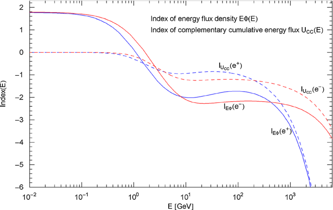
The Index function $I_{E\Phi } (E)$ of the electronic and positronic energy flux densities $E\Phi (E)$ as well as the Index $I_{{U_{{{\text{CC}}}} }} (E)$ of the complementary cumulative energy fluxes $U_{{{\text{CC}}}} (E)$ are shown in Fig. 26. The Index curves are calculated by way of (4.13) and (4.14) (with the regressed particle flux density $\Phi (E)$ in (4.1) and Table 3) and depict the energy dependence of the Log–Log slope of the electronic/positronic $E\Phi (E)$ and $U_{{{\text{CC}}}} (E)$ in Figs. 24 and 25. The simple power-law approximations of $E\Phi (E)$ and $U_{{{\text{CC}}}} (E)$ shown in these figures as black dashed straight lines seem to be quite suitable in the intermediate energy range, but the Index functions in Fig. 26 show a varying spectral slope, including Log–Log inflection points (in Figs. 24 and 25) at energies where the Index curves have local extrema, cf. Appendix A.

Index functions of the electronic/positronic energy flux density $E\Phi (E)$ and complementary cumulative energy flux $U_{{{\text{CC}}}} (E)$. The solid curves (red/blue for electrons/positrons) show the Index $I_{E\Phi } (E)$ of the energy flux density, cf. (4.13), and the dashed curves depict the Index $I_{{U_{{{\text{CC}}}} }} (E)$ of the complementary cumulative energy flux, cf. (4.14). The Index functions are calculated from the regressed electron/positron fluxes in (4.1) and Table 3 and represent the Log–Log slope of the energy flux densities in Fig. 24 and complementary cumulative energy fluxes in Fig. 25. This is the counterpart to Fig. 23, where the Index functions of the particle flux densities and associated survival functions are plotted

Full size image

In Sect. 3, we demonstrated that multiply broken power-law densities can accurately reproduce the fine structure of electrical resistivity data of metals, covering temperatures up to the melting point. We also used Index functions defined as slope parameter of Log–Log plots to compare the resistivity curves with scaling predictions of electron–electron and electron–phonon scattering, which are $T^{2}$ and $T^{5}$ power laws at low temperature. We found significant deviations from power-law scaling with integer exponents. And even in the classical high-temperature regime close to the melting point, the linear temperature scaling of the electrical resistivity suggested by the Drude model is idealized, since the empirical scaling exponent is consistently larger than one, cf. Sections 3.1–3.3, or, in the case of ferromagnets, substantially smaller than one above the Curie temperature, cf. Section 3.4. The Bloch–Grüneisen formula [26, 27] interpolating between a $T^{5}$ scaling at low temperature and linear scaling in the classical regime is also not an accurate description of resistivity, as it neither reproduces the empirical high- and low-temperature scaling nor the inflection points visible in Log–Log plots of the resistivities at intermediate temperatures. Inflection points can be spotted by plotting the Index functions of the regressed resistivities, since Log–Log inflection points correspond to local extrema of the Index functions.

In the examples discussed in Sects. 3.1–3.4, the electrical resistivity data (as well as the depicted temperature intervals in the figures) were truncated at the melting point, where a discontinuity in the resistivity emerges. At temperatures close to the melting point, the data sets indicate simple (but non-integer) power-law scaling, as illustrated by the Index functions, which become nearly constant at high temperature. As we considered only the temperature interval of the solid phase, there was no need to consider smooth gradual cutoffs for the broken power laws used in the regression.

In Sect. 4, we discussed the modeling of cosmic-ray electron and positron spectra with multiply broken power laws. The measured fluxes exhibit faster than power-law decay at high energy. Weibull and lognormal cutoff factors, actually generalizations thereof, were introduced in Sect. 2.2 to obtain an adaptable crossover from a power-law slope to (stretched or compressed) exponential or lognormal decay. A rescaling of the empirical flux densities in Figs. 16 and 18 indicated two spectral breaks between the power-law segments, before the exponential decay sets in, for positrons and electrons alike. The electronic and positronic survival functions depicted in Figs, 19, 20, 21, 22 and the complementary cumulative energy fluxes in Fig. 25 (both inferred from the regressed flux densities) show substantial spectral variation, quantified by the Index functions in Figs. 23 and 26.

Even though power-law scaling laws are attractive for their technical simplicity and often admit derivation from ‘first principles,’ they tend to be approximative when applied to extended data sets stretching over several logarithmic decades. Examples for that are discussed in Sect. 4. The Log–Log plots of the positron and electron fluxes in Figs. 15 and 17 and the survival functions in Figs. 19 and 21 all suggest power-law scaling over a wide energy range, and the respective goodness-of-fit parameters in Tables 5 and 6 seem to indicate that as well. However, a rescaling of the data sets with the energy variable as in Figs. 16, 18, 20 and 22 tells otherwise, the straight power-law slope is gone, and two closely spaced peaks emerge. The rescaling compresses the flux variation, which ranges over eight or nine logarithmic decades in Figs. 15 and 17, and is reduced to two decades in the rescaled plots in Figs. 16 and 18. Goodness-of-fit parameters are constructed as averages over the data set and do not guarantee uniform accuracy of the fit.

In Sect. 3, the integer power-law scaling laws for the electrical resistivity, derived from first principles (that is electron–phonon and electron–electron scattering at low temperature), have also been found to be approximative when compared to precision data of high-purity samples. The resistivity plots and Index functions of (anti-)ferromagnets are also qualitatively different from dia- and paramagnetic materials, the Néel and Curie transitions clearly showing in Figs. 5, 11 and 13, and, in the case of iron, also the structural transitions above the Curie temperature.

In the review [3], twenty-four large data sets, from word counts via earthquake intensities and bird surveys to website traffic, were scrutinized in search of power-law tails. In many cases, power-law decay could be identified, but very few of these data sets qualify as power laws over the full data range, showing distinct break points and curvature in Log–Log plots, as is the case in the examples discussed here. The tail ends of large data sets can usually be modeled as power-law tails or by (stretched or compressed) exponentials or lognormal cutoffs, cf. Section 2.2. Occasionally, more than one of these options is considered, since the data points tend to get increasingly sparse and scattered at the tail ends; especially the distinction between power-law and lognormal decay (see Appendix A) can become difficult in this case, cf. e.g., Refs. [17, 18]. But the actual problem is to model an extended data set over the full data range, which is the topic of this paper.

Accurate modeling of a large data set exhibiting several peaks and break points in Log–Log plots is likely to require a multi-parameter distribution. To make this practically viable, it is crucial to have a good initial guess for the parameters in the (nonlinear) least-squares regression. A systematic way to find an initial guess for the fitting parameters of the multiply broken power law (2.1) is outlined in Sect. 4.1, by making use of the factorization of the distribution and the asymptotic limits of the individual factors. Here, we have tried to show, by explicit examples, that the broken power-law distribution (2.1) in conjunction with the cutoff factors in Sect. 2.2 is sufficiently adaptable to model large data sets stretching over several logarithmic decades.

Affiliations

1. Sechsschimmelgasse 1 / 21-22, A-1090, Vienna, Austria

   Roman Tomaschitz

Corresponding author

Correspondence to Roman Tomaschitz.

Appendix A: Log–Log and Lin-Log coordinates, power-law slopes, lognormals, and Index functions

A positive function $y = f(x)$ in linear coordinates $x,y \ge 0$ is transformed into logarithmic coordinates (denoted by a hat) $x = 10^{{\hat{x}}}$, $y = 10^{{\hat{y}}}$ by

where ${\text{Log(}}x) = \log x/\log 10$ denotes the decadic logarithm. Conversely, a function $\hat{y} = g(\hat{x})$ in Log–Log representation is converted via $\hat{x} = {\text{Log(}}x)$, $\hat{y} = {\text{Log(}}y)$ into linear coordinates $x,y \ge 0$ by

To obtain a tangent line in a double-logarithmic plot, we note $\hat{y}^{\prime}(\hat{x}) = xf^{\prime}(x)/f(x)$, according to (A.1). The Log–Log tangent at $\hat{x}_{0} = \log x_{0} /\log 10$, $\hat{y}_{0} = \log f(x_{0} )/\log 10$, reads $\hat{y} = \alpha \hat{x} + a$, with slope $\alpha = x_{0} f^{\prime}(x_{0} )/f(x_{0} )$ and vertical intercept $a = (\log f(x_{0} ) - \alpha \log x_{0} )/\log 10$. This Log–Log tangent corresponds to the power law $y = 10^{a} x^{\alpha }$ in linear coordinates, cf. (A.2). As for Log–Log inflection points, we note $\hat{y}^{\prime\prime}(\hat{x})/\log 10 = (xf^{\prime}(x)/f(x))^{\prime}x$; if $\hat{x}_{0}$ is an inflection point of a Log–Log plot, the derivative of $xf^{\prime}(x)/f(x)$ vanishes at $x_{0} = 10^{{\hat{x}_{0} }}$. Local minima and maxima of $xf^{\prime}(x)/f(x)$ thus indicate inflection points of $\hat{y}(\hat{x})$ in (A.1). In general, a Log–Log inflection point does not have a counterpart in linear representation.

Example 1

$y = Ax^{{\alpha + \beta \log x + \gamma \log^{2} x + \cdots }}$, where the ellipsis in the exponent indicates possible higher powers of $\log x$, so that $y^{\prime} = (\alpha + 2\beta \log x + 3\gamma \log^{2} x + \cdots )y/x$. If $\gamma = 0$, $\beta < 0$, this is a lognormal distribution. In Log–Log coordinates, we obtain a polynomial,

Lognormals are second-order polynomials in Log–Log representation, and a power law ($\beta = \gamma = 0$) is Log–Log linear. Thus, the regression of a lognormal distribution just amounts to fitting a second-order polynomial to a Log–Log plot of the data set, and a power law implies linear regression.

Example 2

$y = Ax^{\alpha } \exp ( - (x/d)^{\delta } )$, with $A,d,\delta > 0$, so that $y^{\prime} = (\alpha - \delta (x/d)^{\delta } )y/x$. In Log–Log coordinates, this Weibull distribution reads

the power-law factor $Ax^{\alpha }$ becomes a linear function, and the cutoff factor emerges as subtracted exponential in this representation.

To define Index functionals, we start with a function $y = f(x)$, $x > 0$, which reads, in Lin-Log coordinates, $y = f(10^{{\hat{x}}} )$, the logarithmic coordinate being denoted by a hat, $\hat{x} = {\text{Log(}}x)$. The function $y = I_{f} (x) = xf^{\prime}(x)/f(x)$ is the linear representation of the Log–Log slope (Index) of $f(x)$, see after (A.2). The Lin-Log representation of the Index $I_{f} (x)$ is $y = I_{f} (10^{{\hat{x}}} ) = 10^{{\hat{x}}} f^{\prime}(10^{{\hat{x}}} )/f(10^{{\hat{x}}} )$.

For instance, a lognormal $f(x) = Ax^{\alpha + \beta \log x}$, $\beta < 0$, has the Index function $y = I_{f} (10^{{\hat{x}}} ) = \alpha + 2\beta \hat{x}\log 10$. Thus, the Index of a lognormal is linear in Lin-Log representation, and the Index of a power law is constant. Conversely, if the Index $I_{f} (x)$ is constant or linear (with negative slope) in Lin-Log representation $y = I_{f} (10^{{\hat{x}}} )$, then $f(x)$ is a power law or lognormal, cf. Example 1 above, where $y = I_{f} (x) = \alpha + 2\beta \log x + \cdots$. A Weibull distribution, $f(x) = Ax^{\alpha } \exp ( - (x/d)^{\delta } )$, has the Index function $y = I_{f} (x) = \alpha - \delta (x/d)^{\delta } = \alpha - \delta {\text{e}}^{{\delta \hat{x}\log 10}} /d^{\delta }$, cf. Example 2 above.

Reprints and Permissions