Caloric and isothermal equations of state of solids: empirical modeling with multiply broken power-law densities

Roman Tomaschitz

doi:10.1007/s00339-019-3256-7

Applied Physics A

February 2020, 126:102 | Cite as

Caloric and isothermal equations of state of solids: empirical modeling with multiply broken power-law densities

Roman Tomaschitz

Roman Tomaschitz
- 1
Email authorView author's OrcID profile

1.ViennaAustria

Article

First Online: 16 January 2020

Abstract

Empirical equations of state (EoSs) are developed for solids, applicable over extended temperature and pressure ranges. The EoSs are modeled as multiply broken power laws, in closed form without the use of ascending series expansions; their general analytic structure is explained and specific examples are studied. The caloric EoS is put to test with two carbon allotropes, diamond and graphite, as well as vitreous silica. To this end, least-squares fits of broken power-law densities are performed to heat capacity data covering several logarithmic decades in temperature, the high- and low-temperature regimes and especially the intermediate temperature range where the Debye theory is of limited accuracy. The analytic fits of the heat capacities are then temperature integrated to obtain the entropy and caloric EoS, i.e. the internal energy. Multiply broken power laws are also employed to model the isothermal EoSs of metals (Al, Cu, Mo, Ta, Au, W, Pt) at ambient temperature, over a pressure range up to several hundred GPa. In the case of copper, the empirical pressure range is extended into the TPa interval with data points from DFT calculations. For each metal, the parameters defining the isothermal EoS (i.e. the density–pressure relation) are inferred by nonlinear regression. The analytic pressure dependence of the compression modulus of each metal is obtained as well, over the full data range.

Keywords

Multi-parameter equation of state (EoS) Caloric EoS of carbon allotropes Specific heat of vitreous silica Thermal EoS and compression modulus of metals High-pressure regime Multiply broken power laws

1 Introduction

The aim of this paper is to develop analytic equations of state (EoSs) for solids which can reproduce empirical data sets covering several orders in temperature and pressure, including the extended crossovers between the asymptotic low and high pressure and temperature regimes. The proposed EoSs are multiply broken power laws, which do not involve truncated series expansions in density, pressure or temperature (frequently used in empirical EoSs, cf. e.g. the reviews [1, 2, 3, 4, 5]) and are, therefore, equally suitable for the mentioned asymptotic regions.

At first, we study caloric EoSs, i.e. the temperature dependence of the internal energy, obtained by integration of the isochoric heat capacity. We work out three specific examples, obtaining closed analytic expressions for the heat capacities of diamond, graphite and vitreous silica by least-squares regression. The isochoric heat capacities are structured as multiply broken power laws [6, 7, 8],

C_{V} (T) = b_{0} T^{β_{0}} \prod_{k = 1}^{n} {(1 + (T / b_{k})^{β_{k} / | η_{k} |})}^{η_{k}}

$C_{V} (T) = b_{0} T^{{\beta_{0} }} \prod\limits_{k = 1}^{n} {\left( {1 + (T/b_{k} )^{{\beta_{k} /\left| {\eta_{k} } \right|}} } \right)^{\eta_{k}} }$

(1)

with positive amplitudes

b_{0}

$b_{0}$ and

b_{k}

$b_{k}$ ,

k = 1, \dots, n

$k = 1, \ldots ,n$ , and

b_{k} << b_{k + 1}

$b_{k} < < b_{k + 1}$ . The exponents

β_{k}

$\beta_{k}$ ,

k = 1, \dots, n

$k = 1, \ldots ,n$ are positive,

β_{0}

$\beta_{0}$ is real, and the exponents

η_{k}

$\eta_{k}$ can be positive or negative.

C_{V} (T)

$C_{V} (T)$ is analytic on the positive real axis and consists of

n + 1

$n + 1$ approximate power-law segments,

\propto T^{β_{0}}

$\propto T^{{\beta_{0} }}$ ,

T^{β_{0} + β_{1} sign (η_{1})}, \dots, T^{β_{0} + \sum_{k = 1}^{n} β_{k} sign (η_{k})}

$T^{{\beta_{0} + \beta_{1} {\text{sign}}(\eta_{1} )}} , \ldots ,T^{{\beta_{0} + \sum\nolimits_{k = 1}^{n} {\beta_{k} {\text{sign}}(\eta_{k} )} }}$ in the intervals

T << b_{1}

$T < < b_{1}$ ,

b_{1} << T << b_{2}, \dots, b_{n} << T

$b_{1} < < T < < b_{2} , \ldots ,b_{n} < < T$ , respectively. The amplitudes

b_{k}

$b_{k}$ define the break points between the power-law segments and the exponents

η_{k}

$\eta_{k}$ determine the extent of the transitional regions. Power laws in log–log plots appear as approximately straight segments, and the exponents

η_{k}

$\eta_{k}$ determine the extent of the transitional regions between the power-law segments.

The isochoric heat capacities of diamond, graphite and vitreous ${\text{SiO}}_{ 2}$ , discussed in Sect. 2, are special cases of the broken power-law density (1). In the case of diamond, $C_{V} (T)$ interpolates between the constant Dulong–Petit high-temperature limit and the Debye $T^{3}$ low-temperature slope. In the intermediate temperature range, the broken power law (1) is sufficiently adaptable to model deviations from the Debye theory such as the boson peaks of glasses. In the case of graphite, $C_{V} (T)$ interpolates between the linear low-temperature slope of the degenerate electron gas and the classical Dulong–Petit regime, and in the case of the ${\text{SiO}}_{2}$ glass, the linear low-temperature slope is replaced by a power law with non-integer index close to one, generated by a fermionic two-level system. In the latter two examples, a phononic cubic temperature slope does not emerge in the empirical data sets, as the low-temperature regime is dominated by Fermi systems.

In recent years, new phenomenological EoSs have been proposed to model density–pressure data sets obtained from Hugoniot shock compression of, for instance, alkali metals [9, 10], alkaline earths [11], aluminum [12, 13, 14], iron [15], copper [16], tin [17] and tungsten [18], to mention but a few. In the second part of this paper, multiply broken power laws are employed as isothermal EoSs of metals, with emphasis on the high-pressure (GPa and TPa) regime. In this case, the pressure dependence of the mass density

ρ

$\rho$ has the analytic shape

ρ (P) = ρ_{0} \prod_{k = 1}^{n} {(1 + P / b_{k})}^{η_{k}}

$\rho (P) = \rho_{0} \prod\limits_{k = 1}^{n} {\left( {1 + P/b_{k} } \right)^{{ \, \eta_{k} }} }$

(2)

with positive amplitudes

ρ_{0}

$\rho_{0}$ ,

b_{k}

$b_{k}$ ,

b_{k} << b_{k + 1}

$b_{k} < < b_{k + 1}$ , and real exponents

η_{k}

$\eta_{k}$ ,

k = 1, \dots, n

$k = 1, \ldots ,n$ . These parameters are temperature dependent, but will be treated as constants in the examples studied here, at ambient temperature of 300 K. Density (2) consists of

n + 1

$n + 1$ power-law segments,

\propto 1

$\propto 1$ ,

P^{η_{1}}, \dots, P^{\sum_{k = 1}^{n} η_{k}}

$P^{{\eta_{1} }} , \ldots ,P^{{\sum\nolimits_{k = 1}^{n} {\eta_{k} } }}$ , in the intervals

P << b_{1}

$P < < b_{1}$ ,

b_{1} << P << b_{2}, \dots, b_{n} << P

$b_{1} < < P < < b_{2} , \ldots ,b_{n} < < P$ . In contrast to the broken power law (1), we have put

β_{0} = 0

$\beta_{0} = 0$ and

β_{k} = | η_{k} |

$\beta_{k} = \left| {\eta_{k} } \right|$ in (2), so that

ρ (P)

$\rho (P)$ is analytic at

P = 0

$P = 0$ , which is essential to model the compression modulus in the low-pressure range consistent with ultrasonic measurements. When discussing the compression modulus in Sect. 3, we will also need the logarithmic derivative of density (2),

ρ^{'} (P) / ρ (P) = \sum_{k = 1}^{n} η_{k} / (P + b_{k})

$\rho^{\prime}(P)/\rho (P) = \sum\nolimits_{k = 1}^{n} {\eta_{k} /(P + b_{k} )}$ , to show how the low-pressure limit of EoS (2) is related to the Murnaghan EoS [19, 20, 21, 22, 23, 24].

In Sect. 3, the EoS (2) will be put to test by performing least-squares fits to high-pressure data sets of Al, Cu, Mo, Ta, Au, W, and Pt, which cover an extended pressure range, from ambient (zero) pressure to several hundred GPa [25, 26, 27]. In the case of copper, the available experimental pressure range (up to 450 GPa [26]) will be extended with data sets obtained from DFT calculations [28]. The least-squares fit of the EoS of copper then covers pressures reaching 60 TPa. In Sect. 4, we present our conclusions.

2 Heat capacity, caloric EoS, and entropy of diamond, graphite and vitreous silica

In this section, the modeling of empirical heat capacity data by multiply broken power-law densities is discussed. Two carbon allotropes, diamond and graphite, and a glass,

{v - SiO}_{2}

${\text{v - SiO}}_{ 2}$ , are studied as specific examples. Explicit formulas for the molar isochoric heat capacities are obtained by nonlinear least-squares regression, cf. Figs. 1, 2 and 3. Comparisons with the Debye theory are depicted in Fig. 4. The temperature variation of the internal energy and entropy variables obtained from the regressed heat capacities is shown in Fig. 5. Alternative attempts to find caloric EoSs for diamond and graphite are discussed in Refs. [29, 30, 31, 32] and references therein.

Fig. 1
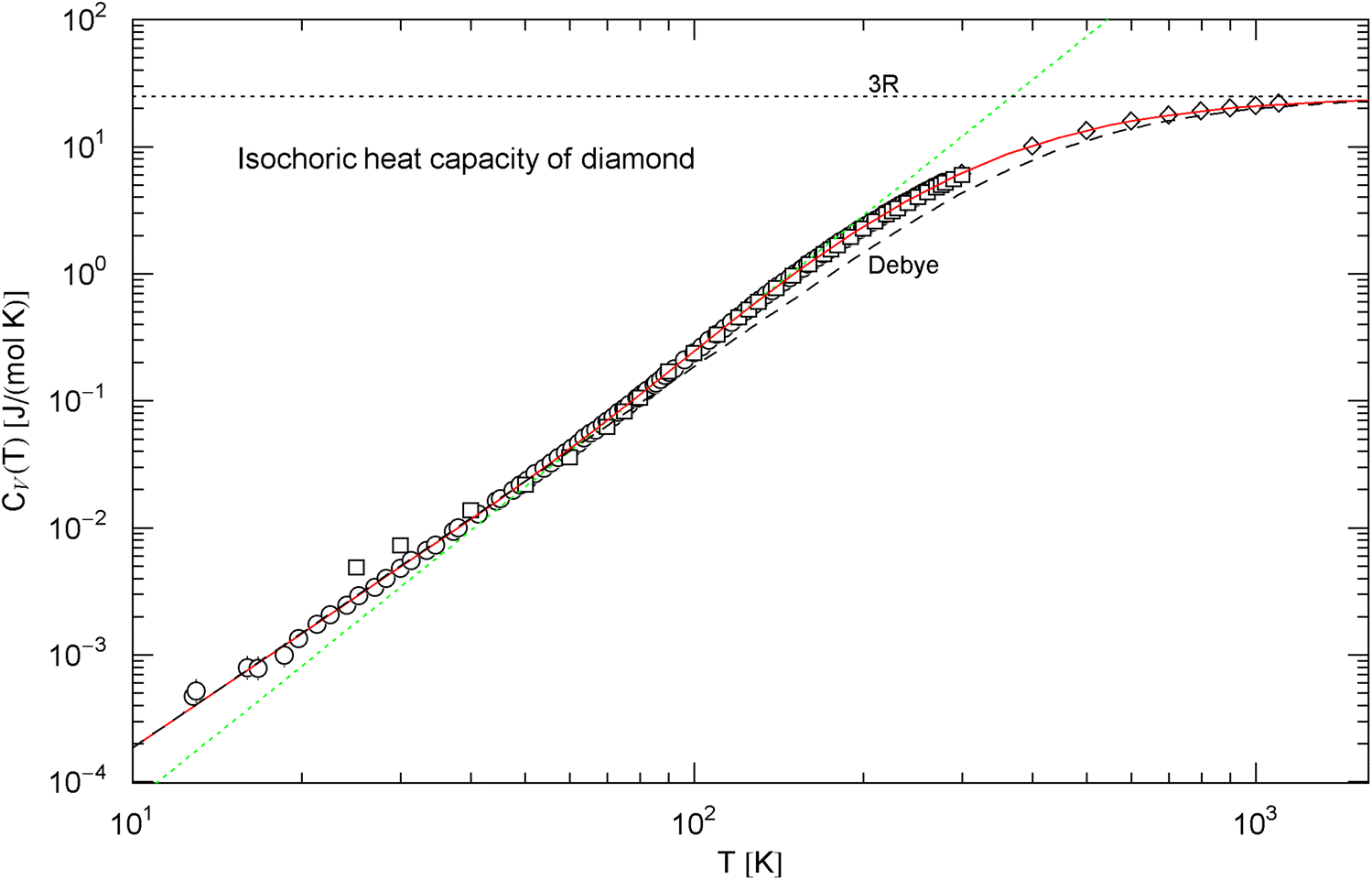
Isochoric heat capacity of diamond, cf. Sect. 2.1. Data points from Ref. [33] (circles), Ref. [34] (squares) and Ref. [35] (diamonds). The $\chi_{{}}^{2}$ fit (solid red curve) is performed with $C_{V}^{{}} (T)$ in (3), the fitting parameters are recorded in Table 1. For comparison, the black dashed curve is the Debye approximation (4), with constant Debye temperature of $\theta_{\text{diamond}} = 2186{\text{ K}}$ . The classical $3R$ Dulong–Petit limit is indicated by the black dotted line. The green dotted straight line depicts the tangent $cT^{\kappa }$ at the inflection point ( $T = 95.53\,{\text{K}}$ , $C_{V}^{{}} = 0.2085\,{\text{J/}}({\text{mol K)}}$ ), with slope $\kappa = 3. 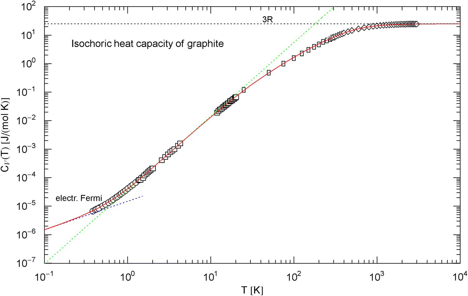5 4 7$ and amplitude $c = 1.972 \times 10^{ - 8} \,{\text{J/}}({\text{mol K}}^{1 + \kappa } )$

Fig. 2
Isochoric heat capacity of graphite, cf. Section 2.2. Data points from Ref. [36] (circles, Madagascar natural graphite), Ref. [37] (squares, Canadian natural graphite), Ref. [38] (rectangles, Acheson graphite), and Ref. [39] (diamonds, Acheson graphite). The experimental isobaric $C_{P}^{{}}$ data points have been converted into isochoric $C_{V}^{{}}$ points, cf. (6). The $\chi_{{}}^{2}$ fit (red solid curve) is performed with the analytic broken power law $C_{V}^{{}} (T)$ in (7), the fitting parameters are listed in Table 1. The dotted blue asymptote $C_{V}^{{}} \sim \;b_{0} T$ is the low-temperature limit of the heat capacity of the electron plasma. The $C_{V}^{{}} (T)$ curve has an inflection point at $T = 3.146\,{\text{K}}$ , $C_{V}^{{}} = 7.170 \times 10^{ - 4} \,{\text{J/}}({\text{mol}}\,{\text{K)}}$ . The dotted green line is the tangent $cT^{\kappa }$ at the inflection point, with amplitude $c = 3. 7 0 2\times 10^{ - 5} \,{\text{J/}}({\text{mol}}\,{\text{K}}^{1 + \kappa } )$ and slope $\kappa = 2. 5 8 6$ , which is the maximum slope attained. See also Fig. 4 for the Debye approximation

Fig. 3
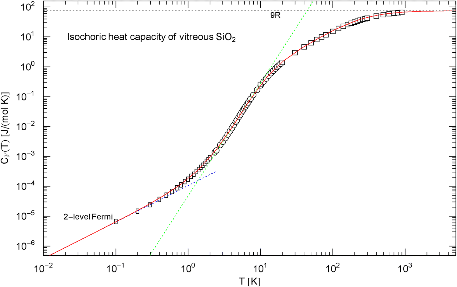
Isochoric heat capacity of ${\text{v - SiO}}_{2}$ , cf. Section 2.3. Data points from Ref. [45] (rectangles), Ref. [46] (circles), and Ref. [47] (squares). The least-squares fit (red solid curve) is performed with the broken power law $C_{V}^{{}} (T)$ in (8), the fitting parameters are recorded in Table 1. The classical $9R$ limit is indicated by the black dotted line. The dotted blue low-temperature asymptote $C_{V}^{{}} \sim \;b_{0} T^{1.22}$ depicts the heat capacity of the two-level Fermi system discussed in Sect. 2.3, which dominates the phononic heat capacity at low temperature. The tangent $cT^{\kappa }$ at the inflection point ( $T = 5.240\,{\text{K}}$ , $C_{V}^{{}} = 2.480 \times 10^{ - 2} \,{\text{J/}}({\text{mol K)}}$ ) has slope $\kappa = 3. 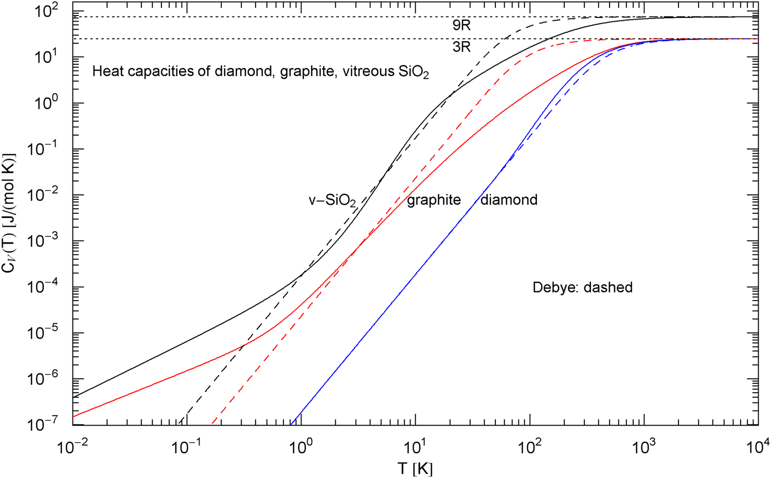7 7 0$ and amplitude $c = 4.815 \times 10^{ - 5} \,{\text{J/}}({\text{mol}}\,{\text{K}}^{1 + \kappa } )$

Fig. 4
Comparison of the molar isochoric heat capacities $C_{V}^{{}} (T)$ of diamond, graphite and vitreous silica. The blue, red and black solid curves show the broken power laws $C_{V}^{{}} (T)$ in (3), (7) and (8), respectively, with fitting parameters in Table 1. (The fits are depicted in Figs. 1, 2 and 3). The dashed curves are the Debye heat capacities, cf. (4). The Debye temperature of diamond is $\theta_{\text{diamond}} = 2186\,{\text{K}}$ ( $c_{D} = b_{0}$ , cf. (4) and Table 1), inferred from the low-temperature limit $C_{V} \sim \;b_{0} T^{3}$ of the broken power law (3). The Debye temperatures $\theta_{\text{graphite}} = 438.7\,{\text{K}}$ and $\theta_{{{\text{v - SiO}}_{2} }} = 323.4\,{\text{K}}$ have been chosen so that the Debye heat capacity (4) intersects the fitted $C_{V}^{{}} (T)$ curves at their inflection point, since the empirical heat capacities of graphite and ${\text{v - SiO}}_{2}$ do not exhibit a $T^{3}$ slope in any temperature range

Fig. 5
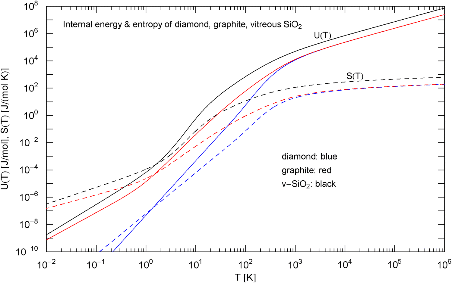
Caloric EoS $U(T) = \int_{0}^{T} {C_{V} {\text{d}}T}$ and molar entropy $S(T) = \int_{0}^{T} {(C_{V} /T){\text{d}}T}$ of diamond, graphite and vitreous silica, cf. (5). The caloric EoSs (thermal component of the internal energy) are depicted as solid curves, the entropies as dashed ones. At high temperature, $U(T) \propto T$ and the entropy diverges logarithmically. The isochoric heat capacities in the integrands are defined in (3), (7) and (8), with fitting parameters in Table 1. The low-temperature slopes read $U(T) \propto T^{{1 + \beta_{0} }}$ and $S(T) \propto T^{{\beta_{0} }}$ , with exponent $\beta_{0}$ in Table 1

2.1 Diamond

We perform a

χ_{}^{2}

$\chi_{{}}^{2}$ fit to the available data sets [33, 34, 35] of the diamond heat capacity, depicted in the double-logarithmic plot in Fig. 1, by employing a broken power law of type (1) as isochoric heat capacity,

C_{V}^{} (T) = b_{0} T^{3} (1 + (T / b_{1})^{β_{1} / η_{1}})^{η_{1}} \frac{1}{(1 + (T / b_{2})^{β_{2} / η_{2}})^{η_{2}}}

$C_{V}^{{}} (T) = b_{0} T^{3} (1 + (T/b_{1} )^{{\beta_{1} /\eta_{1} }} )^{{\eta_{1} }} \frac{1}{{(1 + (T/b_{2} )^{{\beta_{2} /\eta_{2} }} )^{{\eta_{2} }} }}$

(3)

with amplitudes

b_{1} << b_{2}

$b_{1} < < b_{2}$ . The exponents

β_{i}

$\beta_{i}$ ,

η_{i}

$\eta_{i}$ ,

i = 1, 2

$i = 1,2$ are positive, and

β_{2} = 3 + β_{1}

$\beta_{2} = 3 + \beta_{1}$ , so that the classical Dulong–Petit limit

C_{V} (T \to \infty) \sim 3 R

$C_{V} (T \to \infty )\sim 3R$ is recovered, with gas constant

R = 8.314 J/(K mol)

$R = 8.314{\text{ J/(K mol)}}$ . This limit also requires amplitudes in (3) related by

b_{0} = 3 R b_{1}^{β_{1}} / b_{2}^{β_{2}}

$b_{0} = 3Rb_{1}^{{\beta_{1} }} /b_{2}^{{\beta_{2} }}$ . The low-temperature limit is

C_{V} (T \to 0) \sim b_{0} T^{3}

$C_{V} (T \to 0)\sim \;b_{0} T^{3}$ ; the units used are

C_{V}^{} [J / (K mol)]

$C_{V}^{{}} [{\text{J}}/({\text{K mol)}}]$ ,

b_{0} [{J/(K}^{4} mol)]

$b_{0} [ {\text{J/(K}}^{4} {\text{ mol)]}}$ , and

b_{i} [K]

$b_{i} [{\text{K}}]$ .

Broken power laws composed of multiple factors

(1 + (T / b_{i})^{β_{i} / | η_{i} |})^{η_{i}}

$(1 + (T/b_{i} )^{{\beta_{i} /\left| {\eta_{i} } \right|}} )^{{\eta_{i} }}$ are quite efficient for data sets stretching over several decades in temperature, as demonstrated in the subsequent examples. In (3), we have three successive power laws,

\propto T^{3}

$\propto T^{3}$ ,

T^{3 + β_{1}}

$T^{{3 + \beta_{1} }}$ ,

T^{3 + β_{1} - β_{2}}

$T^{{3 + \beta_{1} - \beta_{2} }}$ , in the intervals

T << b_{1}

$T < < b_{1}$ ,

b_{1} << T << b_{2}

$b_{1} < < T < < b_{2}$ and

b_{2} << T

$b_{2} < < T$ , respectively, which appear as approximately straight segments in log–log plots, and the exponents

η_{1}

$\eta_{1}$ ,

η_{2}

$\eta_{2}$ determine the transitional regions around the break points

b_{1}

$b_{1}$ and

b_{2}

$b_{2}$ . The parameters

b_{1}

$b_{1}$ ,

b_{2}

$b_{2}$ ,

η_{1}

$\eta_{1}$ ,

η_{2}

$\eta_{2}$ and

β_{1}

$\beta_{1}$ obtained from the least-squares fit are recorded in Table 1. In contrast to the Debye heat capacity, cf. (4), the heat capacity of diamond exhibits an inflection point in the crossover region between the low- and high-temperature regimes, see Fig. 1; the tangent of

C_{V}

$C_{V}$ at the inflection point is shown as green dotted line depicting the power law

\propto T^{3. 547}

$\propto T^{ 3. 5 4 7}$ .

Table 1

Fitting parameters of the molar isochoric heat capacity $C_{V} (T)$ of diamond, graphite and vitreous silica, see Figs. 1, 2 and 3

	Diamond	Graphite	${\text{v - SiO}}_{ 2}$
$b_{0}$	$1.8605 \times 10^{ - 7}$	$1. 4 8 4 3\times 10^{ - 5}$	$1. 0 6 1 8\times 10^{ - 4}$
$b_{1} [{\text{K}}]$	67.435	0.60277	2.6677
$b_{2} [{\text{K}}]$	282.02	40.466	10.585
$b_{3} [{\text{K}}]$	–	562.35	247.30
$\beta_{0}$	3	1	1.22
$\beta_{1}$	1.2496	1.6796	4.3172
$\beta_{2}$	$\beta_{0} + \beta_{1}$	1.3235	4.0656
$\beta_{3}$	–	$\beta_{0} + \beta_{1} - \beta_{2}$	$\beta_{0} + \beta_{1} - \beta_{2}$
$\eta_{1}$	0.30536	0.69130	2.7558
$\eta_{2}$	2.1816	1.1347	1.7243
$\eta_{3}$	–	0.56727	0.93528
$\chi^{2}$	0.144	0.0539	0.0635
dof	117–5	114–8	78–8
SE	0.070	0.070	0.431
$1 - R^{2}$	$2.41 \times 10^{ - 4}$	$5.55 \times 10^{ - 5}$	$5.16 \times 10^{ - 4}$

The listed parameters (amplitudes $b_{i}$ , exponents $\beta_{i}$ , $\eta_{i}$ ) define the multiply broken power laws (3) (for diamond), (7) (graphite) and (8) (vitreous ${\text{SiO}}_{2}$ ) representing the empirical heat capacities. Some of these parameters are interrelated, cf. Sect. 2. $b_{0}$ is in units of $\text{J}/(\text{K}^{1+{\beta}_0} \,\text{mol})$ . Also recorded are the minimum of the least-squares functional $\chi^{2} = \sum\nolimits_{i = 1}^{N} {(C_{V} (T_{i} ) - C_{Vi} )^{2} /C_{Vi}^{2} }$ and the degrees of freedom (dof: number $N$ of data points $(T_{i} ,C_{Vi} )$ minus number of independent fitting parameters). The standard error of the fits, ${\text{SE}} = (\sum\nolimits_{i = 1}^{N} {(C_{V} (T_{i} ) - C_{Vi} )^{2} /N)^{1/2} }$ , and the coefficient of determination, $R^{2} = 1 - \sum\nolimits_{i = 1}^{N} {(C_{V} (T_{i} ) - C_{Vi} )^{2} } /(N\sigma^{2} )$ , with sample variance $\sigma^{2} = \sum\nolimits_{i = 1}^{N} {(C_{Vi} - \bar{C}_{V} )^{2} /N}$ and mean $\bar{C}_{V} = \sum\nolimits_{i = 1}^{N} {C_{Vi} } /N$ , are listed as well

In Figs. 1 and 4, we have also indicated the Debye approximation,

\begin{aligned} C_{D} (T) & = 9 n_{a / m} R [4 D (θ / T) - \frac{θ / T}{e^{θ / T} - 1}], D (x) := \frac{1}{x^{3}} \int_{0}^{x} \frac{y^{3} d y}{e^{y} - 1}, \\ θ & = {(\frac{12}{5} π^{4} \frac{n_{a / m} R}{c_{D}})}^{1 / 3} . \end{aligned}

$\begin{aligned} C_{D} (T) & = 9n_{a/m} R\left[ {4D(\theta /T) - \frac{\theta /T}{{{\text{e}}^{\theta /T} - 1}}} \right],\quad D(x): = \frac{1}{{x^{3} }}\int\limits_{0}^{x} {\frac{{y^{3} {\text{d}}y}}{{{\text{e}}^{y} - 1}}} , \\ \theta & = \left( {\frac{12}{5}\pi^{4} \frac{{n_{a/m} R}}{{c_{D} }}} \right)^{1/3} . \\ \end{aligned}$

(4)

The asymptotic limits of the Debye function are $D(x > > 1)\sim \;\pi^{4} /(15x^{3} )$ and $D(x < < 1)\sim 1/3$ , so that $C_{D} (T \to 0)\sim \;c_{D} T^{3}$ and $C_{D} (T \to \infty )\sim 3n_{a/m} R$ , where $n_{a/m}$ denotes the number of atoms per molecule. The units are $c_{D} [ {\text{J/(K}}^{4} {\text{ mol)]}}$ and $C_{D} [ {\text{J}}/({\text{K mol)]}}$ as above. The amplitude $c_{D}$ is taken from the least-squares fit of $C_{V} (T)$ in (3), $c_{D} = b_{0}$ , cf. Table 1, to recover the cubic low-temperature slope. Accordingly, the Debye temperature (4) of diamond is $\theta = 2186{\text{ K}}$ . The low-temperature amplitude $c_{D}$ is the only adjustable parameter of the Debye heat capacity, so that it is not surprising that the Debye approximation becomes inaccurate in the crossover region.

The temperature dependence of the caloric EoS (molar internal energy with zero-point energy subtracted) and molar entropy of diamond,

U (T) [J / mol] = \int_{0}^{T} C_{V} d T, S (T) [J / (K mol)] = \int_{0}^{T} \frac{C_{V}}{T} d T

$U(T)[{\text{J}}/{\text{ mol]}} = \int\limits_{0}^{T} {C_{V} {\text{d}}T} ,\quad S(T)[{\text{J}}/({\text{K mol)}}] = \int\limits_{0}^{T} {\frac{{C_{V} }}{T}{\text{d}}T}$

(5)

is shown in Fig. 5, calculated by substituting

C_{V} (T)

$C_{V} (T)$ in (3) with fitting parameters recorded in Table 1.

2.2 Graphite

The heat capacity data of graphite tabulated in the experimental papers [36, 37, 38, 39] refer to the isobaric heat capacity

C_{P}

$C_{P}$ . The conversion of isobaric (at ambient pressure) to isochoric heat capacities

C_{V}

$C_{V}$ is done with the approximate formula

C_{V} \approx C_{P} / (1 + 0.526 T α_{⊥} (T))

$C_{V} \approx C_{P} /(1 + 0.526 \, T\alpha_{ \bot } (T))$ , where

0.526

$0.526$ is the dimensionless Grüneisen constant of graphite [40] and

α_{⊥}

$\alpha_{ \bot }$ the thermal expansion coefficient perpendicular to the basal plane, cf. Refs. [40, 41, 42],

\begin{aligned} α_{⊥} (0 \leq T \leq 80) = 5.35 \times 10^{- 9} T^{2} - 3.755 \times 10^{- 11} T^{3}, \\ \begin{aligned} α_{⊥} (80 \leq T \leq 273) & = 2.435 \times 10^{- 7} T - 7.69 \times 10^{- 10} T^{2} \\ + 8.875 \times 10^{- 13} T^{3}, \end{aligned} \\ α_{⊥} (273 \leq T \leq 1100) = 2.722 \times 10^{- 5} + 3.05 \times 10^{- 9} (T - 273), \\ α_{⊥} (1100 \leq T \leq 3000) = 2.975 \times 10^{- 5} + 9.604 \times 10^{- 9} (T - 1100) . \end{aligned}

$\begin{aligned} & \alpha_{ \bot } (0 \le T \le 80) = 5.35 \times 10^{ - 9} T^{2} - 3.755 \times 10^{ - 11} T^{3} , \\ & \begin{aligned}\alpha_{ \bot } (80 \le T \le 273) &= 2.435 \times 10^{ - 7} T - 7.69 \times 10^{ - 10} T^{2} \\&\quad+ 8.875 \times 10^{ - 13} T^{3} ,\end{aligned} \\ & \alpha_{ \bot } (273 \le T \le 1100) = 2.722 \times 10^{ - 5} + 3.05 \times 10^{ - 9} (T - 273), \\ & \alpha_{ \bot } (1100 \le T \le 3000) = 2.975 \times 10^{ - 5} + 9.604 \times 10^{ - 9} (T - 1100). \\ \end{aligned}$

(6)

The units are $\alpha_{ \bot } [1/{\text{K}}]$ and $T[{\text{K}}]$ . The expansion $\alpha_{||}$ in the basal plane is negligible compared with $\alpha_{ \bot }$ . In the case of diamond, cf. Sect. 2.1, the conversion to isochoric heat capacities has already been done in the experimental papers. In the case of vitreous silica, cf. Sect. 2.3, $C_{V} \approx C_{P}$ in the temperature range of the available data points.

The heat capacity of graphite has an electronic and a phonon component, cf. Fig. 2; at low temperature, the linear electronic heat capacity overpowers the phonon component. For the least-squares fit depicted in Fig. 2, we use a broken power law similarly structured as in (3):

\begin{aligned} C_{V}^{} (T) & = b_{0} T (1 + (T / b_{1})^{β_{1} / η_{1}})^{η_{1}} \\ \times \frac{1}{(1 + (T / b_{2})^{β_{2} / η_{2}})^{η_{2}}} \frac{1}{(1 + (T / b_{3})^{β_{3} / η_{3}})^{η_{3}}}, \end{aligned}

$\begin{aligned} C_{V}^{{}} (T)& = b_{0} T(1 + (T/b_{1} )^{{\beta_{1} /\eta_{1} }} )^{{\eta_{1} }} \\&\quad\times\frac{1}{{(1 + (T/b_{2} )^{{\beta_{2} /\eta_{2} }} )^{{\eta_{2} }} }}\frac{1}{{(1 + (T/b_{3} )^{{\beta_{3} /\eta_{3} }} )^{{\eta_{3} }} }} , \end{aligned}$

(7)

where the factors are ordered by increasing magnitude of the amplitudes,

b_{1} << b_{2} << b_{3}

$b_{1} < < b_{2} < < b_{3}$ , and the exponents

β_{i}

$\beta_{i}$ ,

η_{i}

$\eta_{i}$ ,

i = 1, 2, 3

$i = 1,2,3$ , are positive. We put

β_{3} = 1 + β_{1} - β_{2}

$\beta_{3} = 1 + \beta_{1} - \beta_{2}$ so that

C_{V} (T \to \infty) \sim 3 R

$C_{V} (T \to \infty )\sim 3R$ , which also requires amplitudes related by

b_{0} [{J/(K}^{2} mol)] = 3 R b_{1}^{β_{1}} / (b_{2}^{β_{2}} b_{3}^{β_{3}})

$b_{0} [ {\text{J/(K}}^{2} {\text{ mol)]}} = 3Rb_{1}^{{\beta_{1} }} /(b_{2}^{{\beta_{2} }} b_{3}^{{\beta_{3} }} )$ . The fitting parameters are

b_{i}

$b_{i}$ ,

η_{i}

$\eta_{i}$ ,

i = 1, 2, 3

$i = 1,2,3$ , and

β_{1}

$\beta_{1}$ ,

β_{2}

$\beta_{2}$ , cf. Table 1. The tangent at the inflection point of

C_{V}^{} (T) [J / (K mol)]

$C_{V}^{{}} (T) [ {\text{J}}/({\text{K mol)]}}$ is depicted as dotted green line

\propto T^{2. 586}

$\propto T^{ 2. 5 8 6}$ in Fig. 2, and the electronic low-temperature asymptote

C_{V}^{} (T) \sim b_{0} T

$C_{V}^{{}} (T)\sim \;b_{0} T$ is also shown in this figure.

There is no indication of a $T^{3}$ slope anywhere to be seen in the data set in Fig. 2. Therefore, we choose the amplitude $c_{D}$ defining the Debye temperature in a way that the low-temperature $T^{3}$ slope of the Debye curve $C_{D} (T)$ [stated in (4)] cuts through the inflection point of the empirical heat capacity $C_{V} (T)$ , see Fig. 4. This gives a Debye temperature of $\theta = 438.7{\text{ K}}$ [with $c_{D} = 2.303 \times 10^{ - 5} \,\text{J}/(\text{K}^{4}\,\text{mol})$ in (4)]. A different choice of $\theta$ would just shift the $T^{3}$ slope parallel to the depicted slope. It is evident from Fig. 4 that the standard Debye approximation (4) cannot give a reasonable fit to the heat capacity of graphite, irrespective of the choice of $\theta$ , except at very high temperature; see also Ref. [41] and references therein for modifications of the Debye theory regarding graphite. The internal energy and entropy functions of graphite are shown in Fig. 5, obtained by integrating the empirical $C_{V}^{{}} (T)$ in (7) (with fitting parameters in Table 1) according to Eq. (5).

2.3 Vitreous ${\text{SiO}}_{2}$

For the heat capacity of vitreous silica [43, 44, 45, 46, 47], we use a broken power law similar to that of graphite:

\begin{aligned} C_{V}^{} (T) & = b_{0} T^{β_{0}} (1 + (T / b_{1})^{β_{1} / η_{1}})^{η_{1}} \\ \times \frac{1}{(1 + (T / b_{2})^{β_{2} / η_{2}})^{η_{2}}} \frac{1}{(1 + (T / b_{3})^{β_{3} / η_{3}})^{η_{3}}}, \end{aligned}

$\begin{aligned} C_{V}^{{}} (T)& = b_{0} T^{{\beta_{0} }} (1 + (T/b_{1} )^{{\beta_{1} /\eta_{1} }} )^{{\eta_{1} }}\\&\quad\times \frac{1}{{(1 + (T/b_{2} )^{{\beta_{2} /\eta_{2} }} )^{{\eta_{2} }} }}\frac{1}{{(1 + (T/b_{3} )^{{\beta_{3} /\eta_{3} }} )^{{\eta_{3} }} }} , \end{aligned}$

(8)

where the positive amplitudes

b_{i} [K]

$b_{i} [{\text{K}}]$ are ordered by increasing magnitude,

b_{1} << b_{2} << b_{3}

$b_{1} < < b_{2} < < b_{3}$ . The exponents

β_{i}

$\beta_{i}$ and

η_{i}

$\eta_{i}$ ,

i = 1, 2, 3

$i = 1,2,3$ , are positive, and we put

β_{3} = β_{0} + β_{1} - β_{2}

$\beta_{3} = \beta_{0} + \beta_{1} - \beta_{2}$ so that

C_{V} (T \to \infty) \sim 9 R

$C_{V} (T \to \infty )\sim 9R$ , which also requires

b_{0} [{J/(K}^{1 + β_{0}} mol)] = 9 R b_{1}^{β_{1}} / (b_{2}^{β_{2}} b_{3}^{β_{3}})

$b_{0} [ {\text{J/(K}}^{{1 + \beta_{0} }} {\text{ mol)]}} = 9Rb_{1}^{{\beta_{1} }} /(b_{2}^{{\beta_{2} }} b_{3}^{{\beta_{3} }} )$ . The data points in Fig. 3 refer to the total heat capacity of the phonons and the fermionic two-level system which dominates the phonon heat capacity of the glass at low temperature [48, 49]. The low-temperature heat capacity of the two-level system is slightly different from linear, with power-law exponent of

β_{0} = 1.22

$\beta_{0} = 1.22$ for

{v - SiO}_{2}

${\text{v - SiO}}_{ 2}$ [43, 44]. In the least-squares fit depicted in Fig. 3, we take this exponent

β_{0}

$\beta_{0}$ as input parameter in (8); the low-temperature limit of (8) is

C_{V} [J / (K mol)] \sim b_{0} T^{β_{0}}

$C_{V} [ {\text{J}}/({\text{K mol)]}}\sim \;b_{0} T^{{\beta_{0} }}$ . The fitting parameters are

b_{i}

$b_{i}$ ,

η_{i}

$\eta_{i}$ ,

i = 1, 2, 3

$i = 1,2,3$ , and

β_{1}

$\beta_{1}$ ,

β_{2}

$\beta_{2}$ , cf. Table 1. The tangent of

C_{V}

$C_{V}$ at the inflection point is shown as dotted green line

\propto T^{3. 770}

$\propto T^{ 3. 7 7 0}$ in Fig. 3.

The Debye approximation $C_{D}^{{}} (T)$ of the ${\text{v - SiO}}_{ 2}$ heat capacity is depicted in Fig. 4, cf. (4). As in the case of graphite, there is no $T^{3}$ slope visible in the measured heat capacity. The Debye temperature $\theta = 323.4{\text{ K}}$ [ $c_{D} = 1.724 \times 10^{ - 4} \,\text{J}/(\text{K}^{4}\,\text{mol})$ in (4)] is chosen so that $C_{D}^{{}} (T)$ intersects the empirical heat capacity $C_{V}^{{}} (T)$ [in (8)] at the inflection point. For comparison, the heat capacities $C_{V}^{{}} (T)$ of diamond and graphite, cf. (3), (7) and Table 1, are also indicated in Fig. 4. The molar internal energy and entropy of ${\text{v - SiO}}_{2}$ are depicted in Fig. 5, calculated via (5) and (8).

To quantify the two-level system defining the heat capacity at low temperature [48, 49], we use a Fermi distribution with zero chemical potential and a power-law mode density. The spectral density and the internal energy then read

d ρ (E) = a_{0} \frac{E^{β_{0} - 1} d E}{e^{E / T} + 1},

${\text{d}}\rho (E) = a_{0} \frac{{E^{{\beta_{0} - 1}} {\text{d}}E}}{{{\text{e}}^{E/T} + 1}} ,$

(9)

U (T) = \int_{0}^{\infty} E d ρ (E) = a_{0} T^{1 + β_{0}} (1 - 2^{- β_{0}}) Γ (1 + β_{0}) ζ (1 + β_{0})

$U(T) = \int\limits_{0}^{\infty } {E{\text{d}}\rho (E} ) = a_{0} T^{{1 + \beta_{0} }} (1 - 2^{{ - \beta_{0} }} )\varGamma (1 + \beta_{0} )\zeta (1 + \beta_{0} )$

(10)

with positive exponent

β_{0}

$\beta_{0}$ and amplitude

a_{0}

$a_{0}$ to be determined from heat capacity measurements.

Γ (x)

$\varGamma (x)$ and

ζ (x)

$\zeta (x)$ denote the gamma function and Riemann zeta function, cf. e.g. Ref. [50], and we have put

ℏ = k_{B} = 1

$\hbar=k_B=1$ . The heat capacity is

C_{V} = U^{'} (T) = (1 + β_{0}) U / T

$C_{V} = U^{\prime}(T) = (1 + \beta_{0} )U/T$ . By comparing with the low-temperature limit

C_{V} \sim b_{0} T^{β_{0}}

$C_{V} \sim \,b_{0} T^{{\beta_{0} }}$ of the empirical heat capacity (8), we can specify the exponent

β_{0} = 1.22

$\beta_{0} = 1.22$ and the amplitude in (9),

a_{0} = \frac{b_{0}}{(1 - 2^{- β_{0}}) Γ (2 + β_{0}) ζ (1 + β_{0})}

$a_{0} = \frac{{b_{0} }}{{(1 - 2^{{ - \beta_{0} }} )\varGamma (2 + \beta_{0} )\zeta (1 + \beta_{0} )}}$

(11)

with

b_{0}

$b_{0}$ in Table 1, so that

a_{0} = 5.089 \times 10^{- 5} {J/(K}^{2.22} mol)

$a_{0} = 5.089 \times 10^{ - 5} {\text{J/(K}}^{2.22} {\text{ mol)}}$ . The partition function is related to the internal energy by

\log Z = a_{0} \int_{0}^{\infty} \log (1 + e^{- E / T}) E^{β_{0} - 1} d E = \frac{1}{β_{0}} \frac{U}{T},

$\log Z = a_{0} \int\limits_{0}^{\infty } {\log (1 + {\text{e}}^{ - E/T} )E^{{\beta_{0} - 1}} {\text{d}}E} = \frac{1}{{\beta_{0} }}\frac{U}{T} ,$

(12)

where we used integration by parts, and the entropy reads

S = \log Z + U / T = C_{V} / β_{0}

$S = \log Z + U/T = C_{V} /\beta_{0}$ .

The spectral density

d ρ (E)

${\text{d}}\rho (E)$ in (9) can be written in the equivalent quasi-particle momentum representation

d \hat{ρ} (p) = \frac{4 π s}{(2 π)^{3}} \frac{p^{2} d p}{e^{E (p) / T} + 1}, U = \int_{0}^{\infty} E (p) d \hat{ρ} (p),

${\text{d}}\hat{\rho }(p) = \frac{4\pi s}{{(2\pi )^{3} }}\frac{{p^{2} {\text{d}}p}}{{{\text{e}}^{E(p)/T} + 1}},\quad U = \int\limits_{0}^{\infty } {E(p){\text{d}}\hat{\rho }(p} ),$

(13)

where

s = 2

$s = 2$ is the spin degeneracy and

E (p) = c_{0} p^{3 / β_{0}}, c_{0} := (\frac{4 π s}{(2 π)^{3}} \frac{β_{0}}{3 a_{0}})^{1 / β_{0}}

$E(p) = c_{0} p^{{3/\beta_{0} }} ,\,c_{0} : = (\frac{4\pi s}{{(2\pi )^{3} }}\frac{{\beta_{0} }}{{3a_{0} }})^{{1/\beta_{0} }}$

(14)

is the power-law dispersion relation. Density (13) can be derived by box quantization; the dispersion relation (14) is to be regarded as the leading order of an ascending power series, and the thermodynamic variables derived from (9) or (13) are asymptotic low-temperature limits.

In Sects. 2.1–2.3, we have studied heat capacities and caloric EoSs obtained by fitting broken power laws (1) to empirical data. In the next section, we will use broken power-law densities to model isothermal EoSs of solids at high pressure, as indicated in (2).

3 Isothermal EoS of metals at high pressure

We start with the Murnaghan EoS $P = (K_{0} /K_{0}^{\prime } )((\rho /\rho_{0} )^{{K_{0}^{\prime } }} - 1)$ , cf. e.g. Refs. [19, 51, 52], where $K_{0}$ denotes the bulk modulus $K(P)$ at zero pressure and $K_{0}^{\prime }$ its pressure derivative at $P = 0$ (practically ambient pressure). $\rho (P)$ denotes the mass density and $\rho_{0}$ the mass density at zero pressure. The temperature dependence of $\rho (P)$ , $K(P)$ and of the constants $K_{0}$ , $K_{0}^{\prime }$ , $\rho_{0}$ will not be explicitly indicated; the data sets studied here refer to a constant ambient temperature of $300\,{\text{K}}$ . Inverting the above EoS, we find $\rho (P)/\rho_{0} = (1 + PK_{0}^{\prime } /K_{0} )^{{1/K_{0}^{\prime } }}$ and the compressibility $\kappa_{T} : = \rho^{\prime}(P)/\rho (P) = 1/(K_{0} + K_{0}^{\prime } P)$ , which gives a linear pressure dependence of the compression modulus $K(P) = 1/\kappa_{T} = K_{0} + K_{0}^{\prime }P$ . Accordingly, $(\rho (P)/\rho^{\prime } (P))_{|P = 0} = K_{0}^{{}} = K(P)_{|P = 0}$ and $(\rho (P)/\rho^{\prime } (P))^{\prime}_{|P = 0} = K_{0}^{\prime } = K^{\prime } (P)_{|P = 0}$ . This linear relation and the Murnaghan EoS are usually applicable up to pressures of a few ${\text{GPa}}$ , cf. e.g. Ref. [53].

To obtain density–pressure relations extending into the high-pressure range, we write the broken power-law density (2) as

\frac{ρ (P)}{ρ_{0}} = {(1 + \frac{{\hat{K}}_{0}^{'}}{{\hat{K}}_{0}} P)}^{1 / {\hat{K}}_{0}^{'}} \prod_{k = 2}^{n} {(1 + P / b_{k})}^{η_{k}},

$\frac{\rho (P)}{{\rho_{0} }} = \left( {1 + \frac{{\hat{K}_{0}^{\prime } }}{{\hat{K}_{0} }}P} \right)^{{1/\hat{K}_{0}^{\prime } }} \prod\limits_{k = 2}^{n} {\left( {1 + P/b_{k} } \right)^{{ \, \eta_{k} }} } ,$

(15)

where we have put

b_{1} = {\hat{K}}_{0} / {\hat{K}}_{0}^{'}

$b_{1} = \hat{K}_{0} /\hat{K}_{0}^{\prime }$ and

η_{1} = 1 / {\hat{K}}_{0}^{'}

$\eta_{1} = 1/\hat{K}_{0}^{\prime }$ . The first factor in (15) is modeled after the inverted Murnaghan EoS. The amplitudes in (15) are ordered according to

b_{k} << b_{k + 1}

$b_{k} < < b_{k + 1}$ , see after (2). For pressures up to several hundred GPa (achievable in current shock compression experiments), two factors [

n = 2

$n = 2$ in (15)] suffice to obtain an accurate density–pressure relation. In this case, the EoS (15) is composed of three successive power laws,

\propto 1

$\propto 1$ ,

P^{1 / \hat{K_{0}^{'}}}

$P^{1/\hat{{K^{\prime}_{0}} }}$ ,

P^{1 / \hat{K_{0}^{'}} + η_{2}}

$P^{{1/\hat{K^{\prime}_{0}} + \eta_{2} }}$ , in the intervals

P << {\hat{K}}_{0} / {\hat{K}}_{0}^{'}

$P < < \hat{K}_{0} /\hat{K}_{0}^{\prime }$ ,

{\hat{K}}_{0} / {\hat{K}}_{0}^{'} << P << b_{2}

$\hat{K}_{0} /\hat{K}_{0}^{\prime } < < P < < b_{2}$ and

b_{2} << P

$b_{2} < < P$ , respectively.

The compression modulus derived from EoS (15) reads

K (P) = \frac{ρ (P)}{ρ^{'} (P)} = \frac{{\hat{K}}_{0} + {\hat{K}}_{0}^{'} P}{1 + Δ (P)}, Δ (P) := ({\hat{K}}_{0} + {\hat{K}}_{0}^{'} P) \sum_{k = 2}^{n} \frac{η_{k}}{b_{k}} \frac{1}{1 + P / b_{k}},

$K(P) = \frac{\rho (P)}{{\rho^{\prime } (P)}} = \frac{{\hat{K}_{0} + \hat{K}_{0}^{\prime } P}}{1 + \Delta (P)},\quad \Delta (P): = (\hat{K}_{0} + \hat{K}_{0}^{\prime } P)\sum\limits_{k = 2}^{n} {\frac{{\eta_{k} }}{{b_{k} }}\frac{1}{{1 + P/b_{k} }}} ,$

(16)

where we made use of the logarithmic derivative of

ρ (P)

$\rho (P)$ stated after (2).

K (P)

$K(P)$ admits a Taylor expansion

K (P) = K_{0} + K_{0}^{'} P + O (P^{2})

$K(P) = K_{0} + {K}_{0}^{\prime } P + {\text{O}}(P^{2} )$ with coefficients

K_{0} = \frac{{\hat{K}}_{0}}{1 + {\hat{K}}_{0} A}, K_{0}^{'} = \frac{{\hat{K}}_{0}^{'} + {\hat{K}}_{0}^{2} B}{(1 + {\hat{K}}_{0} A)^{2}}, A := \sum_{k = 2}^{n} \frac{η_{k}}{b_{k}}, B := \sum_{k = 2}^{n} \frac{η_{k}}{b_{k}^{2}} .

$K_{0} = \frac{{\hat{K}_{0} }}{{1 + \hat{K}_{0} A}},\quad {K}_{0}^{\prime } = \frac{{\hat{K}_{0}^{\prime } + \hat{K}_{0}^{2} B}}{{(1 + \hat{K}_{0} A)^{2} }},\quad A: = \sum\limits_{k = 2}^{n} {\frac{{\eta_{k} }}{{b_{k} }}} ,\quad B: = \sum\limits_{k = 2}^{n} {\frac{{\eta_{k} }}{{b_{k}^{2} }}} .$

(17)

Accordingly, the parameters

{\hat{K}}_{0}

$\hat{K}_{0}$ and

{\hat{K}}_{0}^{'}

$\hat{K}_{0}^{\prime }$ defining the first factor of EoS (15) are related to the bulk modulus at zero pressure,

K_{0}^{} = K (P)_{| P = 0}

$K_{0}^{{}} = K(P)_{|P = 0}$ , and to its derivative

K_{0}^{'} = K^{'} (P)_{| P = 0}

${K}_{0}^{\prime } = K^{\prime } (P)_{|P = 0}$ by

{\hat{K}}_{0} = \frac{K_{0}}{1 - K_{0} A}, \hat{K_{0}^{'}} = \frac{K_{0}^{'} - K_{0}^{2} B}{(1 - K_{0} A)^{2}},

$\hat{K}_{0} = \frac{{K_{0} }}{{1 - K_{0} A}},\quad \hat{K^{\prime}_{0}} = \frac{{{K}_{0}^{\prime } - K_{0}^{2} B}}{{(1 - K_{0} A)^{2} }},$

(18)

which is the inversion of (17). We substitute these relations for

{\hat{K}}_{0}

$\hat{K}_{0}$ and

{\hat{K}}_{0}^{'}

$\hat{K}_{0}^{\prime }$ in EoS (15), so that the first factor of EoS (15) depends on the parameters

K_{0}

$K_{0}$ ,

K_{0}^{'}

$K_{0}^{\prime }$ and

b_{k}

$b_{k}$ ,

η_{k}

$\eta_{k}$ ,

k = 2, \dots, n

$k = 2, \ldots ,n$ . Evidently, if

| K_{0} A | << 1

$\left| {K_{0} A} \right| < < 1$ and

| K_{0}^{2} B / K_{0}^{'} | << 1

$\left| {K_{0}^{2} B/K_{0}^{\prime } } \right| < < 1$ , then

{\hat{K}}_{0} \approx K_{0}

$\hat{K}_{0} \approx K_{0}$ and

{\hat{K}}_{0}^{'} \approx K_{0}^{'}

$\hat{K}_{0}^{\prime } \approx K_{0}^{\prime }$ . The bulk modulus

K_{0}

$K_{0}$ at zero pressure and its derivative

K_{0}^{'}

$K_{0}^{\prime }$ are taken as measured input in EoS (15), inferred from acoustic low-pressure experiments. The amplitudes and exponents

b_{k}

$b_{k}$ ,

η_{k}

$\eta_{k}$ ,

k = 2, \dots, n

$k = 2, \ldots ,n$ in EoS (15) are to be determined by least-squares regression. If ultrasonic measurements of

K_{0}^{'}

$K_{0}^{\prime }$ are not available, we can take

K_{0}^{'}

$K_{0}^{\prime }$ as additional fit parameter, and the same holds for

K_{0}

$K_{0}$ . As mentioned, the EoS (15) with two factors suffices for pressures up to several hundred GPa, so that only two fit parameters

b_{2}

$b_{2}$ ,

η_{2}

$\eta_{2}$ are needed for data sets presently obtainable by shock compression.

We test EoS (15) with pressure isotherms of Al (Fig. 6), Cu (Fig. 7), Mo (Fig. 8), Ta (Fig. 9), Au (Fig. 10), W (Fig. 11) and Pt (Fig. 12), all at ambient temperature of

300 K

$300{\text{ K}}$ . The least-squares fits (red solid curves) are based on EoS (15) (with

n = 2

$n = 2$ and relations (18) substituted) and data sets from Refs. [25, 26, 27]. The fit parameters

b_{2}

$b_{2}$ ,

η_{2}

$\eta_{2}$ and the input parameters

ρ_{0}

$\rho_{0}$ and

K_{0}

$K_{0}$ ,

K_{0}^{'}

$K_{0}^{\prime }$ (the latter two obtained from ultrasonic measurements [54, 55, 56, 57, 58, 59, 60, 61, 62, 63, 64, 65]) as well as the goodness-of-fit parameters (

χ^{2} / dof

$\chi^{2} /{\text{dof}}$ , standard error, determination coefficient) are recorded in Table 2. In the case of Mo and Pt,

K_{0}^{'}

$K_{0}^{\prime }$ is treated as a third fit parameter, for lack of ultrasonic estimates. In Fig. 13, the pressure range of copper (by shockless compression up to 450 GPa [26], cf. Figure 7) has been extended to

60 TPa

$6 0\,{\text{TPa}}$ using data points from DFT calculations [28], in which case a third factor can be specified in EoS (15) (

n = 3

$n = 3$ ), depending on two additional fit parameters

b_{3}

$b_{3}$ ,

η_{3}

$\eta_{3}$ recorded in the last column of Table 2.

Fig. 6
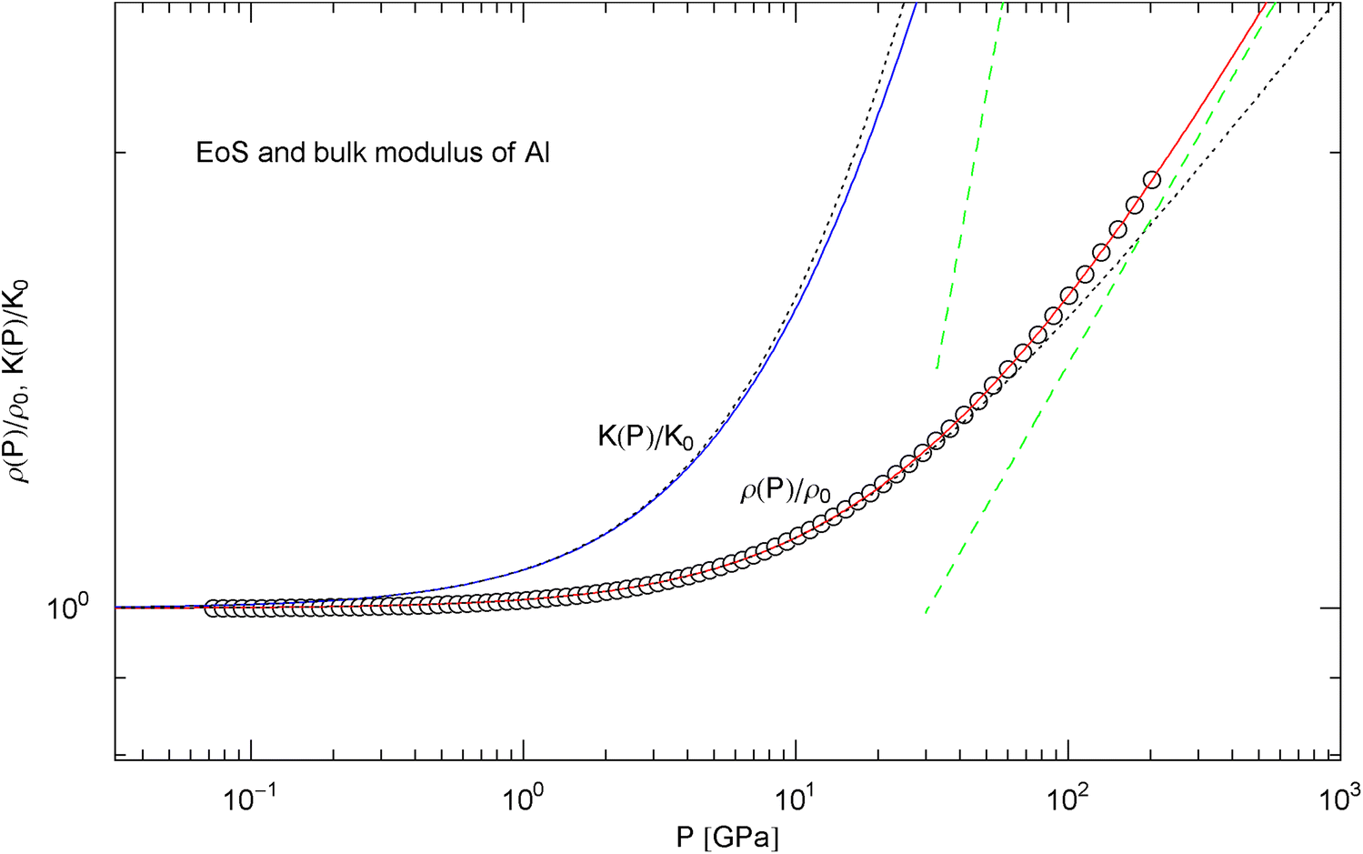
Pressure isotherm at $300{\text{ K}}$ and compression modulus of aluminum. Data points up to 200 GPa (by Hugoniot shock compression) from Ref. [25]. The $\chi_{{}}^{2}$ fit (solid red curve) is performed with the isothermal EoS $\rho (P)$ in (15) ( $n = 2$ ), the fitting parameters $b_{2}$ , $\eta_{2}$ are recorded in Table 2. The solid blue curve depicts the compression modulus $K(P)$ calculated from the fitted EoS, cf. (16). $\rho_{0}$ and $K_{0}$ denote mass density and compression modulus at zero pressure, cf. Table 2. The dashed green lines are asymptotes to $\rho (P)/\rho_{0}$ and $K(P)/K_{0}$ . The dotted black curves depict the Murnaghan approximations of the EoS and compression modulus, cf. after (18), calculated with $K_{0}$ and its derivative $K^{\prime}_{0}$ obtained from ultrasonic measurements, cf. Table 2

Fig. 7
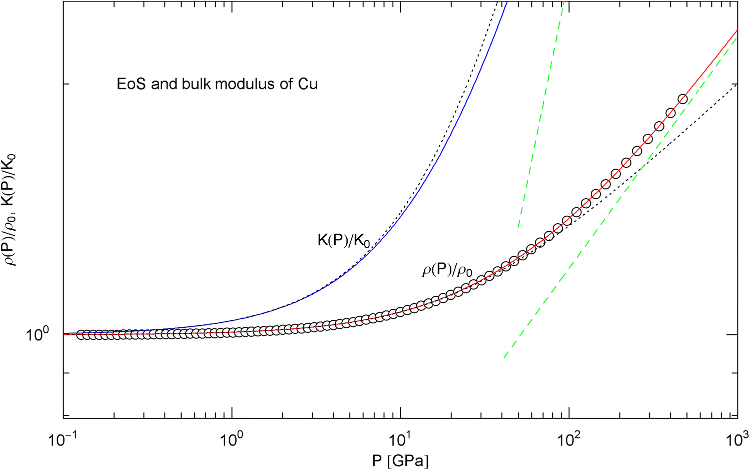
Pressure isotherm and compression modulus of copper. Data points up to 450 GPa (via shockless compression) from Ref. [26]. The caption to Fig. 6 applies. The $\chi_{{}}^{2}$ fit (solid red curve) is performed with EoS $\rho (P)$ in (15), the fitting parameters are listed in Table 2. The solid blue curve shows the compression modulus $K(P)$ , cf. (16). The dashed green lines are asymptotes. The dotted black curves depict the Murnaghan approximations, cf. after (18). See also Fig. 13 for the extension of the EoS into the TPa range

Fig. 8
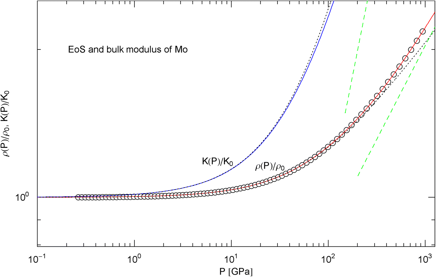
Pressure isotherm and compression modulus of molybdenum. Data points up to 1 TPa (by shock compression) from Ref. [27]. The caption of Fig. 6 applies. The $\chi_{{}}^{2}$ fit (solid red curve) is performed with EoS $\rho (P)$ in (15) and fitting parameters in Table 2. The solid blue curve shows the compression modulus $K(P)$ , cf. (16). The dashed green lines are asymptotes and the dotted black curves depict the Murnaghan approximations

Fig. 9
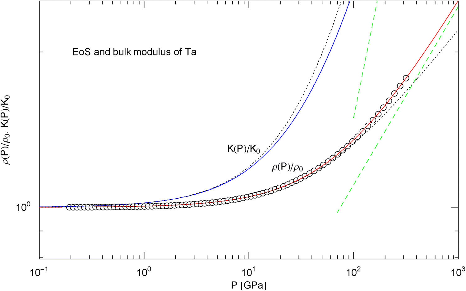
Pressure isotherm and compression modulus of tantalum. Data points up to 300 GPa by shock compression [25]. The $\chi_{{}}^{2}$ fit (solid red curve) is performed with EoS $\rho (P)$ in (15) and fitting parameters in Table 2. The compression modulus $K(P)$ , cf. (16), is depicted as blue solid curve. The dashed green lines are the asymptotes of $\rho (P)/\rho_{0}$ and $K(P)/K_{0}$ . The dotted black curves depict the Murnaghan EoS and the linear compression modulus derived from it, cf. after (18)

Fig. 10
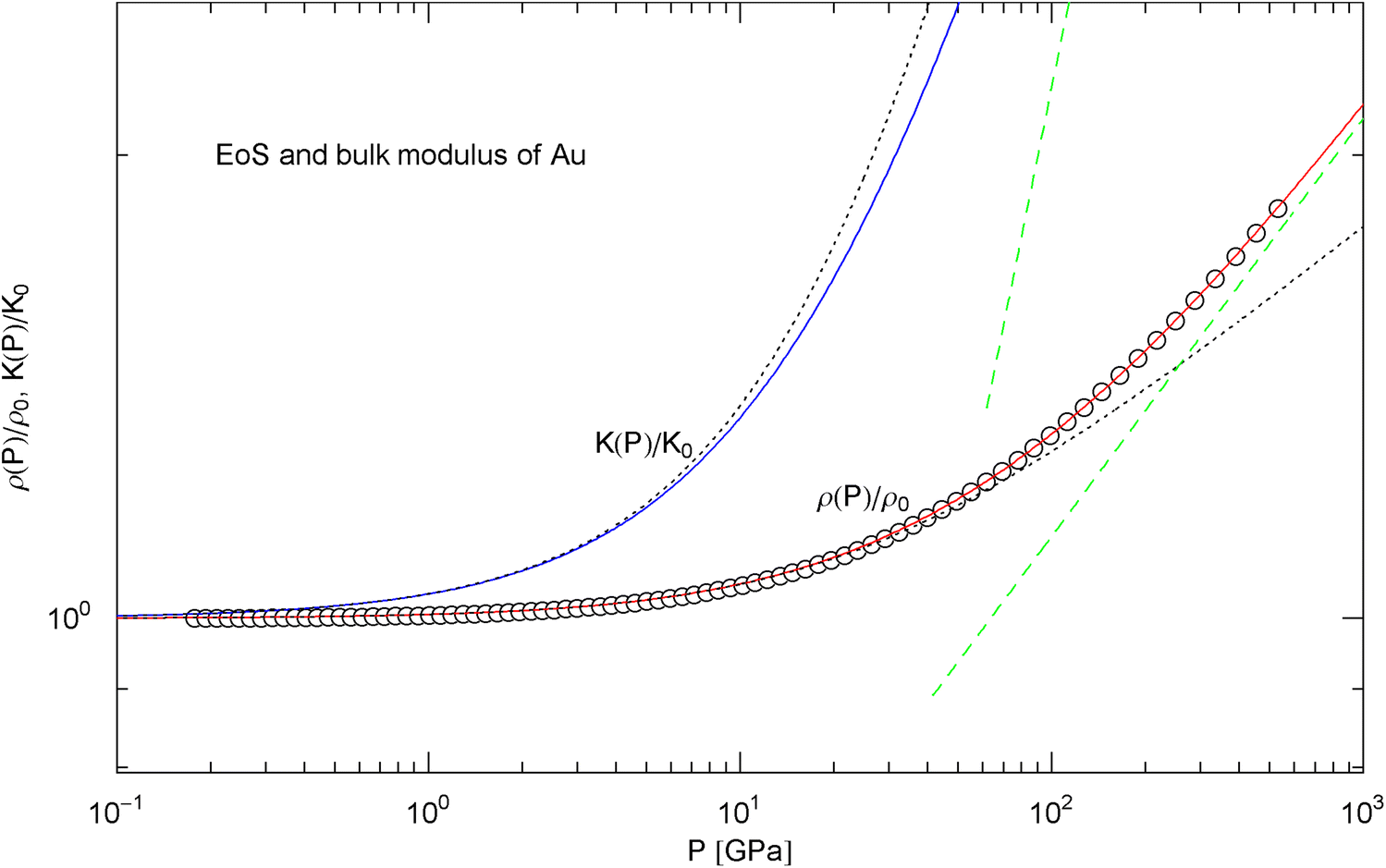
Pressure isotherm at $300{\text{ K}}$ and compression modulus of gold. Data points up to 500 GPa by shock compression [27]. The $\chi_{{}}^{2}$ fit (solid red curve) is performed with EoS $\rho (P)$ in (15), the fitting parameters are recorded in Table 2. The solid blue curve shows the compression modulus $K(P)$ , cf. (16). The dashed green lines are asymptotes and the dotted black curves depict the Murnaghan approximations

Fig. 11
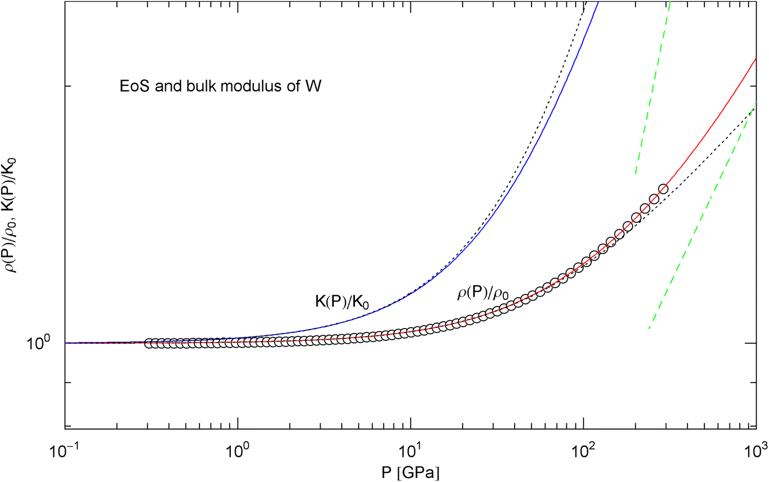
Pressure isotherm at $300{\text{ K}}$ and compression modulus of tungsten. Data points up to 300 GPa by shock compression [25]. The $\chi_{{}}^{2}$ fit (solid red curve) is performed with EoS $\rho (P)$ in (15) and fitting parameters in Table 2. The solid blue curve is the compression modulus $K(P)$ , cf. (16). The dotted black curves depict the Murnaghan EoS and the linear approximation of the compression modulus, cf. after (18). The dashed green lines are asymptotes

Fig. 12
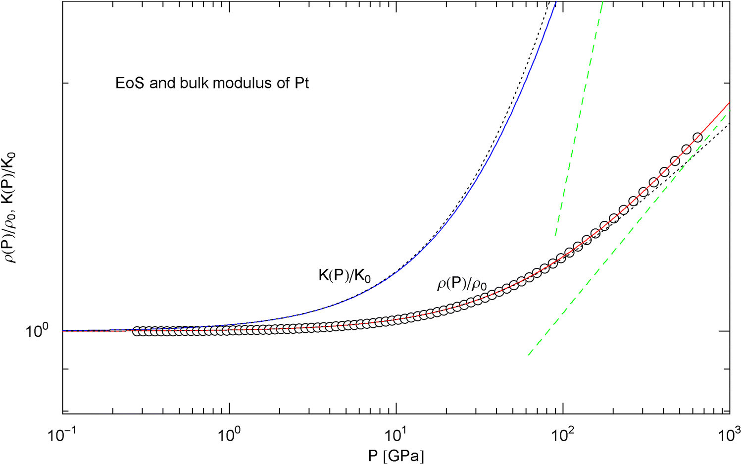
Pressure isotherm and compression modulus of platinum. Data points up to 660 GPa by shock compression [27]. The $\chi_{{}}^{2}$ fit (solid red curve) is performed with EoS $\rho (P)$ in (15), the fitting parameters are recorded in Table 2. The solid blue curve shows the compression modulus $K(P)$ , cf. (16). The dashed green lines are asymptotes and the dotted black curves depict the Murnaghan approximations, cf. after (18)

Table 2

Fitting parameters of the pressure isotherms of Al, Cu, Mo, Ta, Au, W and Pt, at ambient temperature of $300{\text{ K}}$ . The isothermal EoS used for the fits is defined in (15)

	Al	Cu	Mo	Ta	Au	W	Pt	Cu @ TPa
$\rho_{0} [{\text{g}}/{\text{cm}}^{3} ]$	2.707	8.939	10.22	16.67	19.24	19.25	21.41	8.939
$K_{0} [{\text{GPa}}]$	73	133.5	264.87	194	166.7	296	280.03	133.5
$K^{\prime}_{0}$	4.42	5.36	3.7499	3.83	6.23	4.3	5.0886	5.36
$b_{2} [{\text{GPa}}]$	78.084	120.03	612.12	90.405	114.00	531.46	169.13	113.31
$\eta_{2}$	0.13699	0.14094	0.14521	0.28648	0.17773	0.25268	0.10226	0.13916
$b_{3} [{\text{GPa}}]$	–	–	–	–	–	–	–	6507.1
$\eta_{3}$	–	–	–	–	–	–	–	0.15077
$\hat{K}_{0}[{\text{GPa}}]$	83.723	158.32	282.63	503.58	225.24	344.48	337.11	160.28
$\hat{K^{\prime}_{0}}$	5.6564	7.2929	4.2386	16.918	10.680	5.7177	6.9681	7.4471
$\chi^{2}$	$6.06 \times 10^{ - 5}$	$2.53 \times 10^{ - 5}$	$1.68 \times 10^{ - 5}$	$1.02 \times 10^{ - 4}$	$7.75 \times 10^{ - 5}$	$1.27 \times 10^{ - 5}$	$5.00 \times 10^{ - 7}$	$5.40 \times 10^{ - 4}$
dof	82	82	84	80	81	75	78	112
SE	$1.04 \times 10^{ - 3}$	$6.37 \times 10^{ - 4}$	$6.88 \times 10^{ - 4}$	$1.34 \times 10^{ - 3}$	$1.06 \times 10^{ - 3}$	$4.34 \times 10^{ - 4}$	$1.12 \times 10^{ - 4}$	$6.57 \times 10^{ - 3}$
$1 - R^{2}$	$2.26 \times 10^{ - 5}$	$8.56 \times 10^{ - 6}$	$6.23 \times 10^{ - 6}$	$5.22 \times 10^{ - 5}$	$2.76 \times 10^{ - 5}$	$1.20 \times 10^{ - 5}$	$4.21 \times 10^{ - 7}$	$3.57 \times 10^{ - 5}$

The mass density $\rho_{0}$ , cf. Ref. [25], and the bulk modulus $K_{0}$ at zero pressure and its pressure derivative $K^{\prime}_{0}$ inferred from ultrasonic measurements [54, 55, 56, 57, 58, 59, 60, 61, 62, 63, 64, 65] are taken as input parameters. In the case of Mo and Pt, $K^{\prime}_{0}$ is treated as fitting parameter, for lack of acoustic measurements. Otherwise, there are only two fitting parameters in EoS (15) (with $n = 2$ ), the amplitude $b_{2}$ and exponent $\eta_{2}$ defining the second factor of the EoS. The pressure isotherms are depicted in Figs. 6, 7, 8, 9, 10, 11 and 12, covering pressures up to a few hundred GPa (subject to availability of data points). In the last column, we have indicated the parameters of the EoS of copper extended to pressures up to 60 TPa with high-pressure data points from DFT calculations [28], see Fig. 13. In this case, a third factor in EoS (15) can be specified ( $n = 3$ ), depending on two additional fitting parameters $b_{3}$ and $\eta_{3}$ . Also listed are the constants $\hat{K}_{0}$ and $\hat{K^{\prime}_{0}}$ defining the first factor of the EoS (15), which are calculated from the input and fitting parameters according to (17) and (18). The minimum of the least-squares functional $\chi^{2}$ , the degrees of freedom (dof), the standard error ${\text{SE}}$ and determination coefficient $R^{2}$ (see the caption to Table 1) of the least-squares fits in Figs. 6, 7, 8, 9, 10, 11, 12 and 13 are recorded as well

Fig. 13
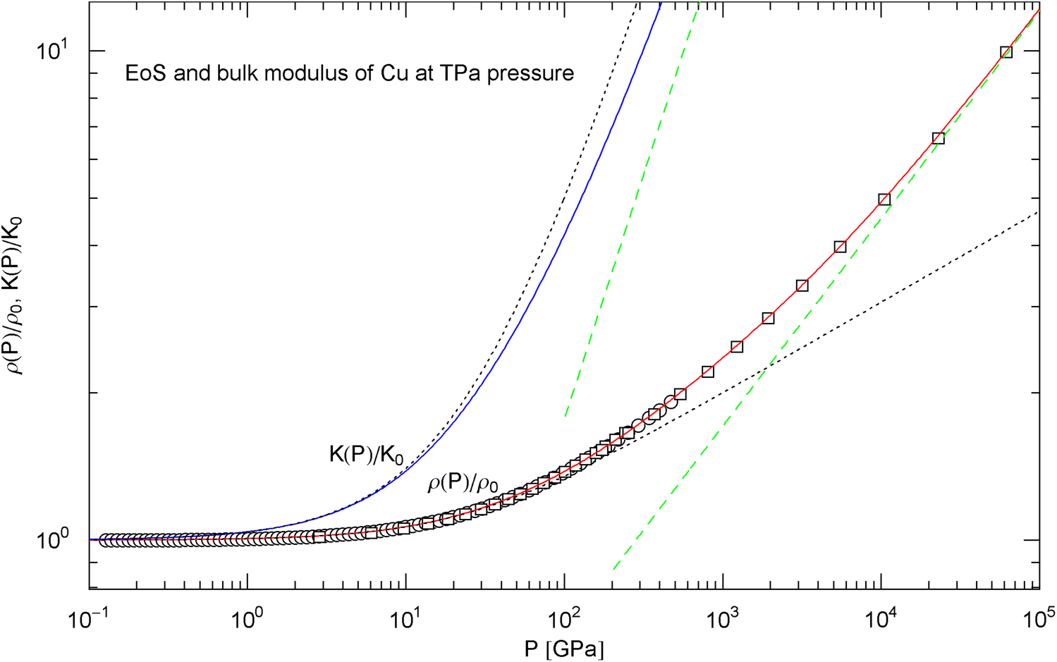
Pressure isotherm at $300{\text{ K}}$ and compression modulus of copper up to 60 TPa. Data points up to 450 GPa (circles) obtained by shockless compression [26] and up to 60 TPa (squares) from DFT calculations [28]. The $\chi_{{}}^{2}$ fit (solid red curve) is performed with the isothermal EoS $\rho (P)$ in (15) (with $n = 3$ ), the fitting parameters are listed in Table 2. The solid blue curve shows the compression modulus $K(P)$ , cf. (16). The dotted black curves depict the Murnaghan EoS and the linear compression modulus derived from it, cf. after (18). The dashed green straight lines indicate the asymptotes of the pressure isotherm and compression modulus

In Figs. 6, 7, 8, 9, 10, 11, 12 and 13, we have also depicted the pressure dependence of the compression modulus $K(P)$ (solid blue curves) defined in (16), using input and fitting parameters of the regressed EoS (15) listed in Table 2. In these figures, we also compare the EoS (15) with the Murnaghan EoS $\rho_{\text{M}} (P)/\rho_{{{\text{M}}0}} = (1 + (K_{0}^{\prime } /K_{0} )P)^{{1/K_{0}^{\prime } }}$ outlined at the beginning of this section [we write here $\rho_{\text{M}} (P)$ and $\rho_{{{\text{M}}0}}$ for density and density at zero pressure to distinguish this EoS from the general EoS in (15)]. The compression modulus $K(P)$ in (16) is also compared with the linear relation $K_{\text{M}} (P) = K_{0} + K_{0}^{\prime } P$ obtained from the Murnaghan EoS. (The linearity of $K_{\text{M}} (P)$ is somewhat hidden in the log–log representation of the figures.) Actually, this linear relation, experimentally verified up to pressures of a few GPa (but usually invalid above 10 GPa, see Figs. 6, 7, 8, 9, 10, 11 and 12) is the starting point when deriving the Murnaghan EoS, by substituting $K_{\text{M}} (P) = \rho_{\text{M}} (P)/\rho^{\prime}_{\text{M}} (P)$ and integrating.

The compression modulus

K (P)

$K(P)$ in (16) coincides with the Murnaghan approximation

K_{M} (P)

$K_{\text{M}} (P)$ in linear order, cf. (17). The EoS (15) is analytic at

P = 0

$P = 0$ and can be expanded in an ascending series,

\frac{ρ (P)}{ρ_{0}} = 1 + \frac{1}{K_{0}} P + \frac{1 - K_{0}^{'}}{2 K_{0}^{2}} P^{2} + \dots

$\frac{\rho (P)}{{\rho_{0} }} = 1 + \frac{1}{{K_{0} }}P + \frac{{1 - K_{0}^{\prime } }}{{2K_{0}^{2} }}P^{2} + \cdots$

(19)

with

K_{0}

$K_{0}$ and

K_{0}^{'}

$K_{0}^{\prime }$ in (17), by making use of the zero pressure identities

(ρ (P) / ρ^{'} (P))_{| P = 0} = K_{0}^{}

$(\rho (P)/\rho^{\prime}(P))_{|P = 0} = K_{0}^{{}}$ and

(ρ (P) / ρ^{'} (P))_{| P = 0}^{'} = K_{0}^{'}

$(\rho (P)/\rho^{\prime } (P))_{|P = 0}^{\prime } = K^{\prime}_{0}$ . The Murnaghan EoS admits the same second-order expansion. As is evident from Figs. 6, 7, 8, 9, 10, 11 and 12, a linear compression modulus is quite accurate up to about 5 GPa, and the Murnaghan approximation of EoS (15) remains valid up to about 50 GPa.

In the opposite high-pressure regime, the leading order of EoS (15) is a power law,

\begin{aligned} ρ (P) \sim a_{\infty} P^{α_{\infty}}, α_{\infty} := \frac{1}{\hat{K_{0}^{'}}} + \sum_{k = 2}^{n} η_{k}, \\ a_{\infty} := ρ_{0} {(\frac{\hat{K_{0}^{'}}}{{\hat{K}}_{0}})}^{1 / \hat{K_{0}^{'}}} \prod_{k = 2}^{n} b_{k}^{- η_{k}}, \end{aligned}

$\begin{aligned}& \rho (P)\sim \;a_{\infty } P^{{\alpha_{\infty } }} ,\quad \alpha_{\infty } : = \frac{1}{{\hat{K^{\prime}_{0}} }} + \sum\limits_{k = 2}^{n} {\eta_{k} } ,\\&\quad a_{\infty } : = \rho_{0} \left( {\frac{{\hat{K^{\prime}_{0}} }}{{\hat{K}_{0} }}} \right)^{{1/\hat{K^{\prime}_{0}} }} \prod\limits_{k = 2}^{n} {b_{k}^{{ - \eta_{k} }} } , \end{aligned}$

(20)

and it is convenient to write

Δ (P)

$\Delta (P)$ in (16) as

Δ (P) = \hat{K_{0}^{'}} (1 + \frac{{\hat{K}}_{0}}{\hat{K_{0}^{'}} P}) \sum_{k = 2}^{n} \frac{η_{k}}{1 + b_{k}^{} / P},

$\Delta (P) = \hat{K^{\prime}_{0}} \left(1 + \frac{{\hat{K}_{0} }}{{\hat{K^{\prime}_{0}} P}}\right)\sum\limits_{k = 2}^{n} {\frac{{\eta_{k} }}{{1 + b_{k}^{{}} /P}}} ,$

(21)

which converges to a constant at high pressure,

Δ (P) = \hat{K_{0}^{'}} \sum_{k = 2}^{n} η_{k} + O (1 / P)

$\Delta (P) = \hat{K^{\prime}_{0}} \sum\nolimits_{k = 2}^{n} {\eta_{k} } + {\text{O}}(1/P)$ . The corresponding asymptotic limits of the compression modulus (16) and its derivative are

K (P) = K_{\infty}^{'} P + O (1)

$K(P) = K^{\prime}_{\infty } P + {\text{O}}(1)$ and

K^{'} (P) = K_{\infty}^{'} + O (1 / P^{2})

$K^{\prime}(P) = K^{\prime}_{\infty } + {\text{O}}(1/P^{2} )$ , where

K_{\infty}^{'} = K^{'} (P)_{| P \to \infty} = 1 / α_{\infty}

$K^{\prime}_{\infty } = K^{\prime}(P)_{|P \to \infty } = 1/\alpha_{\infty }$ with

α_{\infty} (\hat{K_{0}^{'}}, η_{k}) = 1 / \hat{K_{0}^{'}} + \sum_{k = 2}^{n} η_{k}

$\alpha_{\infty } (\hat{K^{\prime}_{0}} ,\eta_{k} ) = 1/\hat{K^{\prime}_{0}} + \sum\nolimits_{k = 2}^{n} {\eta_{k} }$ as defined in (20).

The EoS $\rho (P) \propto P^{3/5}$ of a non-relativistic degenerate electron gas in the Thomas–Fermi free-electron approximation gives $K^{\prime}_{\infty } = 5/3$ [51, 66], leading to the condition $\alpha_{\infty } (\hat{K^{\prime}_{0}} ,\eta_{k} ) = 3/5$ to be satisfied by the exponents $\hat{K^{\prime}_{0}}$ and $\eta_{k}$ in (15) and (20). Application of this relation to the EoS of copper depicted in Fig. 13 (which is accurate up to 60 TPa and based on EoS (15) with $n = 3$ and parameters in Table 2) suggests that an additional factor $\left( {1 + P/b_{4} } \right)^{{ \, \eta_{4} }}$ with $\eta_{4} \approx 0.176$ will be necessary in EoS (15) ( $n = 4$ ) to extend the density–pressure curve beyond 60 TPa. (In the case of an ultra-relativistic degenerate electron plasma, $K^{\prime}_{\infty } = 5/3$ is replaced by $K^{\prime}_{\infty } = 4/3$ , so that $\alpha_{\infty } = 3/4$ .) Phenomenological thermodynamic arguments were used in Refs. [67, 68] to suggest the inequality $K^{\prime}_{\infty } > 5/3$ instead of $K^{\prime}_{\infty } = 5/3$ . In contrast to the positivity of the heat capacities and compressibilities, this is not a necessary equilibrium condition but presumably more realistic for planetary cores than the Thomas–Fermi limit [5, 69]. The inequality $K^{\prime}_{\infty } > 5/3$ weakens the above condition to $\alpha_{\infty } (\hat{K^{\prime}_{0}} ,\eta_{k} ) < 3/5$ and gives the constraint $\eta_{4} < 0.176$ on the exponent of the fourth factor in the ultra-high pressure EoS of copper applicable beyond 60 TPa.

4 Conclusion

The examples discussed in Sects. 2 and 3 demonstrate the efficiency of multiply broken power laws in modeling empirical equations of state of solids. The heat capacities $C_{V} (T)$ and mass densities $\rho (P)$ defined in Sect. 1 are analytic functions composed of power-law segments joint by smooth analytic transitions; they do not involve series expansions, being assembled as products of power-law factors $(1 + (x/b_{k} )^{{\beta_{k} /\left| {\eta_{k} } \right|}} )^{{\eta_{k} }}$ , $k = 1, \ldots ,n$ , cf. (1) and (2), where $x$ stands for the temperature or pressure variable. Broken power laws are particularly suitable to model data sets where pressure or temperature varies over several orders of magnitude, interpolating between different asymptotic regimes. The condition $b_{k} < < b_{k + 1}$ on the amplitudes defining the power-law factors allows us to systematically assemble caloric and isothermal EoSs over an ever increasing temperature or pressure range; since $b_{k} < < b_{k + 1}$ , the factor with amplitude $b_{k + 1}$ does not significantly affect the EoS in the range $x \le b_{k}$ .

In Sect. 2, we discussed three examples of caloric EoSs (of two carbon allotropes and vitreous ${\text{SiO}}_{2}$ ); the corresponding isochoric heat capacities exhibit very different low-temperature power-law scaling and also deviate noticeably from the Debye theory in the intermediate temperature range. The log–log plots in Figs. 1, 2 and 3 depict least-squares fits of the heat capacities [modeled as broken power laws, cf. (3), (7) and (8)] to the respective isochoric data sets of diamond, graphite and ${\text{v - SiO}}_{2}$ . For these materials, heat capacity measurements (including the conversion from isobaric to isochoric heat capacities by way of Grüneisen parameter and thermal expansion coefficient) are available over an extended temperature range covering the low- and high-temperature regimes. As these examples demonstrate, broken power laws are sufficiently adaptable to accurately reproduce the heat capacities over the full empirical temperature range, including features such as the boson peak of the glass in Fig. 4 emerging at around 10 K or the excess heat capacity (as compared to the Debye theory) of diamond peaking at 200 K, cf. Figs. 1 and 4. The analytic heat capacities obtained from the least-squares fits can be temperature integrated to obtain the caloric EoS and entropy variable, see Fig. 5.

In Sect. 3, we discussed isothermal EoSs of specific metals, capable of reproducing high-pressure data sets. The examples studied cover a wide range of mass densities (at ambient pressure), from Al to Pt, cf. Table 2. In contrast to the multiply broken power laws modeling the heat capacities in Sect. 2, which are non-analytic at $T = 0$ , we used broken power laws analytic at zero pressure, cf. (2). The EoS can then be made to converge to the Murnaghan EoS in the low-pressure regime, where the compression modulus is known to vary linearly with pressure. The least-squares fits of the isothermal EoS (15) to high-pressure data sets of Al, Cu, Mo, Ta, Au, W and Pt are depicted in Figs. 6, 7, 8, 9, 10, 11 and 12. In all cases, the fits are uniformly accurate over the full empirical pressure range, from ambient pressure to several hundred GPa. In Fig. 13, the empirical EoS of Cu is extended into the TPa regime, using data points from DFT calculations for the least-squares regression. In Sect. 3, we also explained the implementation of the ultra-high pressure Thomas–Fermi limit into empirical isothermal EoSs defined by multiply broken power laws.

Notes

References

1.
W.B. Holzapfel, High Press. Res. 16, 81 (1998)ADSCrossRefGoogle Scholar
2.
W.B. Holzapfel, Z. Kristallogr. 216, 473 (2001)Google Scholar
3.
J.S. Tse, W.B. Holzapfel, J. Appl. Phys. 104, 043525 (2008)ADSCrossRefGoogle Scholar
4.
J. Hama, K. Suito, J. Phys. Condens. Matter 8, 67 (1996)ADSCrossRefGoogle Scholar
5.
F.D. Stacey, Rep. Prog. Phys. 68, 341 (2005)ADSCrossRefGoogle Scholar
6.
R. Tomaschitz, Physica A (2020). https://doi-org. /10.1016/j.physa.2019.123188 CrossRefGoogle Scholar
7.
R. Tomaschitz, Physica A 483, 438 (2017)ADSMathSciNetCrossRefGoogle Scholar
8.
R. Tomaschitz, Fluid Phase Equilib. 496, 80 (2019)CrossRefGoogle Scholar
9.
K.V. Khishchenko, J. Phys: Conf. Ser. 946, 012082 (2018)Google Scholar
10.
K.V. Khishchenko, J. Phys. Conf. Ser. 1147, 012001 (2019)CrossRefGoogle Scholar
11.
K.V. Khishchenko, Tech. Phys. Lett. 30, 829 (2004)ADSCrossRefGoogle Scholar
12.
D.V. Minakov, P.R. Levashov, K.V. Khishchenko, AIP Conf. Proc. 1426, 836 (2012)ADSCrossRefGoogle Scholar
13.
D.V. Minakov, P.R. Levashov, K.V. Khishchenko, V.E. Fortov, J. Appl. Phys. 115, 223512 (2014)ADSCrossRefGoogle Scholar
14.
M.A. Kadatskiy, K.V. Khishchenko, J. Phys: Conf. Ser. 653, 012079 (2015)Google Scholar
15.
M.A. Kadatskiy, K.V. Khishchenko, J. Phys. Conf. Ser. 774, 012005 (2016)CrossRefGoogle Scholar
16.
M.A. Kadatskiy, K.V. Khishchenko, Phys. Plasmas 25, 112701 (2018)ADSCrossRefGoogle Scholar
17.
K.V. Khishchenko, J. Phys. Conf. Ser. 121, 022025 (2008)CrossRefGoogle Scholar
18.
K.V. Khishchenko, J. Phys. Conf. Ser. 653, 012081 (2015)CrossRefGoogle Scholar
19.
J.R. Macdonald, Rev. Mod. Phys. 38, 669 (1966)ADSCrossRefGoogle Scholar
20.
B.G. Yalcin, Appl. Phys. A 122, 456 (2016)ADSCrossRefGoogle Scholar
21.
S. Khatta, S.K. Tripathi, S. Prakash, Appl. Phys. A 123, 582 (2017)ADSCrossRefGoogle Scholar
22.
M. Kaddes, K. Omri, N. Kouaydi, M. Zemzemi, Appl. Phys. A 124, 518 (2018)ADSCrossRefGoogle Scholar
23.
W. Ouerghui, M.S. Alkhalifah, Appl. Phys. A 125, 374 (2019)ADSCrossRefGoogle Scholar
24.
A. Laroussi, M. Berber, B. Doumi, A. Mokaddem, H. Abid, A. Boudali, H. Bahloul, H. Moujri, Appl. Phys. A 125, 676 (2019)ADSCrossRefGoogle Scholar
25.
A.D. Chijioke, W.J. Nellis, I.F. Silvera, J. Appl. Phys. 98, 073526 (2005)ADSCrossRefGoogle Scholar
26.
R.G. Kraus, J.-P. Davis, C.T. Seagle, D.E. Fratanduono, D.C. Swift, J.L. Brown, J.H. Eggert, Phys. Rev. B 93, 134105 (2016)ADSCrossRefGoogle Scholar
27.
Y. Wang, R. Ahuja, B. Johansson, J. Appl. Phys. 92, 6616 (2002)ADSCrossRefGoogle Scholar
28.
C.W. Greeff, J.C. Boettger, M.J. Graf, J.D. Johnson, J. Phys. Chem. Solids 67, 2033 (2006)ADSCrossRefGoogle Scholar
29.
L.E. Fried, W.M. Howard, Phys. Rev. B 61, 8734 (2000)ADSCrossRefGoogle Scholar
30.
K.V. Khishchenko, V.E. Fortov, I.V. Lomonosov, M.N. Pavlovskii, G.V. Simakov, M.V. Zhernokletov, AIP Conf. Proc. 620, 759 (2002)ADSCrossRefGoogle Scholar
31.
K.V. Khishchenko, V.E. Fortov, I.V. Lomonosov, Int. J. Thermophys. 26, 479 (2005)ADSCrossRefGoogle Scholar
32.
S.Sh. Rekhviashvili, Kh.L. Kunizhev, High Temp. 55, 312 (2017)CrossRefGoogle Scholar
33.
J.E. Desnoyers, J.A. Morrison, Philos. Mag. 3, 42 (1958)ADSCrossRefGoogle Scholar
34.
W. DeSorbo, J. Chem. Phys. 21, 876 (1953)ADSCrossRefGoogle Scholar
35.
A.C. Victor, J. Chem. Phys. 36, 1903 (1962)ADSCrossRefGoogle Scholar
36.
B.J.C. van der Hoeven, P.H. Keesom, Phys. Rev. 130, 1318 (1963)ADSCrossRefGoogle Scholar
37.
W. DeSorbo, G.E. Nichols, J. Phys. Chem. Solids 6, 352 (1958)ADSCrossRefGoogle Scholar
38.
W. DeSorbo, W.W. Tyler, J. Chem. Phys. 21, 1660 (1953)ADSCrossRefGoogle Scholar
39.
M.W. Chase, NIST-JANAF Thermochemical Tables, 4th ed. (AIP, Woodbury, 1998), https://janaf.nist.gov
40.
A.T.D. Butland, R.J. Maddison, J. Nucl. Mater. 49, 45 (1973)ADSCrossRefGoogle Scholar
41.
T. Nihira, T. Iwata, Phys. Rev. B 68, 134305 (2003)ADSCrossRefGoogle Scholar
42.
V.N. Senchenko, R.S. Belikov, J. Phys: Conf. Ser. 891, 012338 (2017)Google Scholar
43.
J.C. Lasjaunias, A. Ravex, M. Vandorpe, S. Hunklinger, Solid State Commun. 17, 1045 (1975)ADSCrossRefGoogle Scholar
44.
R.O. Pohl, in: Amorphous Solids, W.A. Phillips, ed. (Springer, Berlin, 1981)Google Scholar
45.
R.B. Stephens, Phys. Rev. B 8, 2896 (1973)ADSCrossRefGoogle Scholar
46.
P. Flubacher, A.J. Leadbetter, J.A. Morrison, B.P. Stoicheff, J. Phys. Chem. Solids 12, 53 (1959)ADSCrossRefGoogle Scholar
47.
R.C. Lord, J.C. Morrow, J. Chem. Phys. 26, 230 (1957)ADSCrossRefGoogle Scholar
48.
P.W. Anderson, B.I. Halperin, C.M. Varma, Philos. Mag. 25, 1 (1972)ADSCrossRefGoogle Scholar
49.
W.A. Phillips, Rep. Prog. Phys. 50, 1657 (1987)ADSCrossRefGoogle Scholar
50.
I.S. Gradshteyn, I.M. Ryzhik, Table of Integrals, Series, and Products, 8th edn. (Academic Press, Waltham, 2015)zbMATHGoogle Scholar
51.
W.B. Holzapfel, Rep. Prog. Phys. 59, 29 (1996)ADSCrossRefGoogle Scholar
52.
W.B. Holzapfel, High Press. Res. 22, 209 (2002)ADSCrossRefGoogle Scholar
53.
G.M. Amulele, M.H. Manghnani, S. Marriappan, X. Hong, F. Li, X. Qin, H.P. Liermann, J. Appl. Phys. 103, 113522 (2008)ADSCrossRefGoogle Scholar
54.
A. Dewaele, P. Loubeyre, M. Mezouar, Phys. Rev. B 70, 094112 (2004)ADSCrossRefGoogle Scholar
55.
W.B. Holzapfel, High Press. Res. 30, 372 (2010)ADSCrossRefGoogle Scholar
56.
K. Katahara, M. Manghnani, E. Fisher, J. Appl. Phys. 47, 434 (1976)ADSCrossRefGoogle Scholar
57.
K.W. Katahara, M.H. Manghnani, E.S. Fisher, J. Phys. F: Met. Phys. 9, 773 (1979)ADSCrossRefGoogle Scholar
58.
P. van’t-Klooster, N.J. Trappeniers, S.N. Biswas, Physica B + C 97, 65 (1979)Google Scholar
59.
S.N. Biswas, P. van’t-Klooster, N.J. Trappeniers, Physica B + C 103, 235 (1981)Google Scholar
60.
J.L. Tallon, A. Wolfenden, J. Phys. Chem. Solids 40, 831 (1979)ADSCrossRefGoogle Scholar
61.
D. Steinberg, J. Phys. Chem. Solids 43, 1173 (1982)ADSCrossRefGoogle Scholar
62.
W. Holzapfel, M. Hartwig, W. Sievers, J. Phys. Chem. Ref. Data 30, 515 (2001)ADSCrossRefGoogle Scholar
63.
K. Syassen, W.B. Holzapfel, J. Appl. Phys. 49, 4427 (1978)ADSCrossRefGoogle Scholar
64.
K. Takemura, A. Dewaele, Phys. Rev. B 78, 104119 (2008)ADSCrossRefGoogle Scholar
65.
W.B. Holzapfel, M.F. Nicol, High Press. Res. 27, 377 (2007)ADSCrossRefGoogle Scholar
66.
E.E. Salpeter, Astrophys. J. 134, 669 (1961)ADSMathSciNetCrossRefGoogle Scholar
67.
F.D. Stacey, Geophys. J. Int. 143, 621 (2000)ADSCrossRefGoogle Scholar
68.
F.D. Stacey, P.M. Davis, Phys. Earth Planet. Inter. 142, 137 (2004)ADSCrossRefGoogle Scholar
69.
F.D. Stacey, J.H. Hodgkinson, Phys. Earth Planet. Inter. 286, 42 (2019)ADSCrossRefGoogle Scholar

Caloric and isothermal equations of state of solids: empirical modeling with multiply broken power-law densities

Abstract

Keywords

1 Introduction

2 Heat capacity, caloric EoS, and entropy of diamond, graphite and vitreous silica

2.1 Diamond

2.2 Graphite

2.3 Vitreous ${\text{SiO}}_{2}$

3 Isothermal EoS of metals at high pressure

4 Conclusion

Notes

References

Copyright information

Personalised recommendations

Caloric and isothermal equations of state of solids: empirical modeling with multiply broken power-law densities

Abstract

Keywords

1 Introduction

2 Heat capacity, caloric EoS, and entropy of diamond, graphite and vitreous silica

2.1 Diamond

2.2 Graphite

2.3 Vitreous SiO2SiO2 {\text{SiO}}_{2}

3 Isothermal EoS of metals at high pressure

4 Conclusion

Notes

References

Copyright information

Personalised recommendations

2.3 Vitreous ${\text{SiO}}_{2}$